
Energy is a vital material foundation for human production and daily life, and its utilization directly influences the development level of human society. With further reliance on fossil fuels, these resources are projected to be exhausted within a century if the energy structure remains unadjusted, triggering a global energy crisis. To address this, countries worldwide have introduced policies to restructure their energy portfolios. According to the BP Statistical Review of World Energy (2020), global primary energy consumption and incremental changes in 2019 are summarized in the table below, which clearly indicates that renewable energy sources such as solar, wind, and hydroelectric power have gained significant attention in recent years.
| Energy Type | Consumption (EJ) | Growth (EJ) | Share (%) | Growth Share vs. 2018 (%) |
|---|---|---|---|---|
| Oil | 193.0 | -1.6 | 33.1 | -0.8 |
| Natural Gas | 141.5 | 2.8 | 24.2 | 0.2 |
| Coal | 157.9 | -0.9 | 27.0 | -0.5 |
| Renewable Energy | 29.0 | 3.2 | 5.0 | 0.5 |
| Hydropower | 37.6 | 0.3 | 6.4 | 0.0 |
| Nuclear Energy | 24.9 | 0.8 | 4.3 | 0.1 |
| Total | 583.9 | 7.7 | 100 | — |
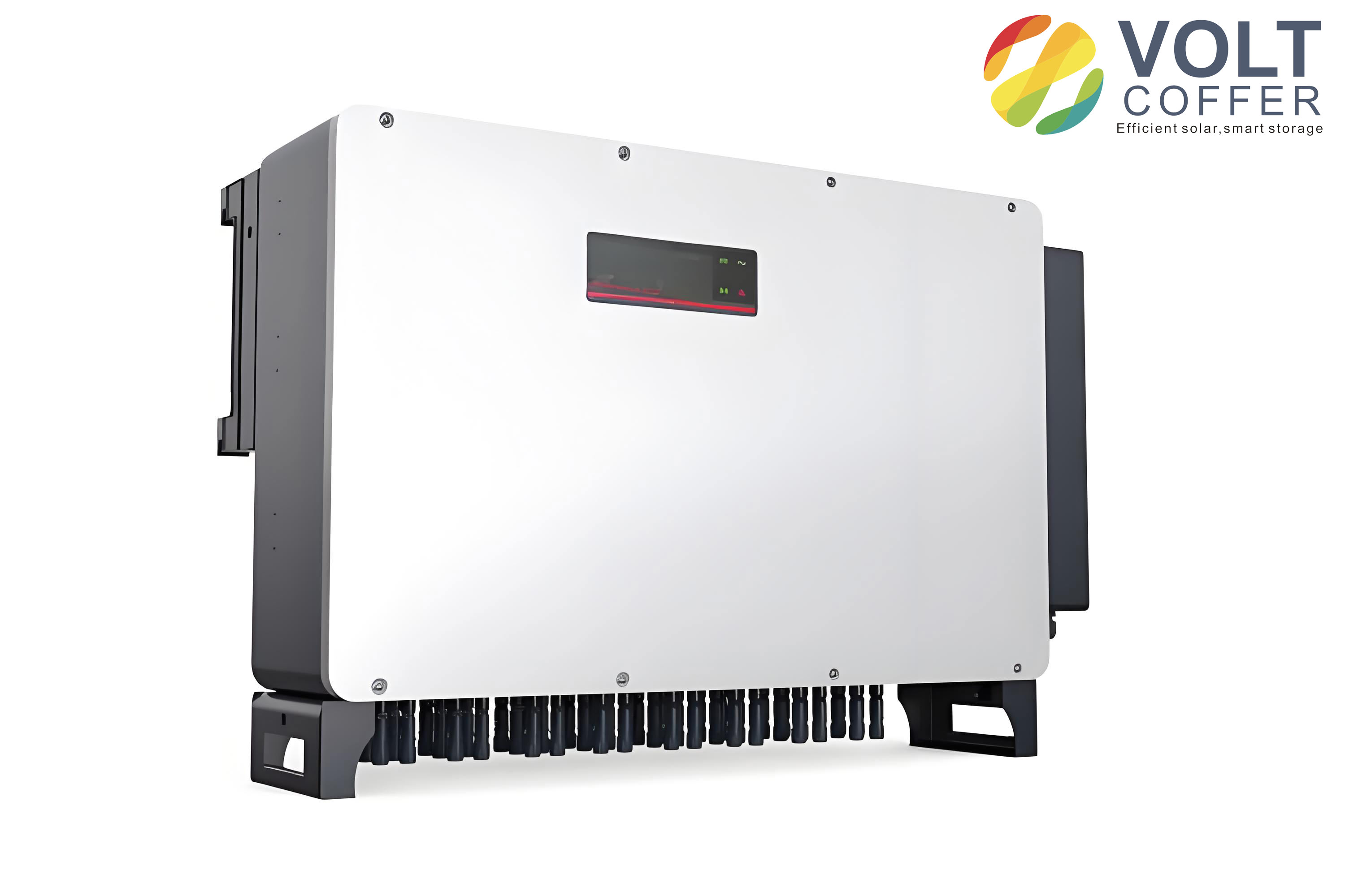
Electric power energy holds a critical position in socialist construction in China and plays an irreplaceable role in the development of various industries. Currently, traditional centralized power generation technology faces increasingly significant challenges during its development, as it not only produces large amounts of harmful gases that pollute the environment but also suffers from difficulties in dispatch and poor reliability. Therefore, existing power generation and transmission modes must be adjusted accordingly. Distributed renewable energy power generation technology has emerged as a key development direction, leveraging the inherent advantages of renewable energy and the unique flexibility of distributed generation to gradually transition from theory to practical application.
The concept of the microgrid was subsequently proposed to further solve the interconnection difficulties between distributed generation systems and the large power grid. A stable, controllable, safe, and reliable microgrid system can generate electricity in a distributed manner and supply power to users. China has exceptionally abundant solar energy resources that provide unique conditions for establishing photovoltaic microgrids. Compared with traditional power generation methods, photovoltaic power generation not only significantly reduces the impact on the environment but also improves the safety and reliability of the power generation system. The inverter, as the core device of photovoltaic power generation, directly affects the system’s safety, reliability, and conversion efficiency. Therefore, research on inverters is of great necessity. In this thesis, I focus on the single-phase solar inverter system. My work investigates the finite control set model predictive control (FCS-MPC) strategy for single-phase solar inverter systems based on mixed logical dynamical (MLD) modeling.
1. Introduction and Research Status
With the further maturity of power electronics inverter technology, the demand for higher total power in power generation systems has increased significantly. There are currently two approaches to solving this problem: one is to increase the power rating of a single inverter; the other is to parallel multiple inverters to increase the total power. Inverter parallel technology has become a key trend in photovoltaic power generation, as it alleviates the weight of photovoltaic modules, fully utilizes distributed power sources at different locations, and enhances system safety and reliability.
The single-phase photovoltaic grid-connected inverter can be categorized into isolated and non-isolated types. The isolated type uses a transformer to separate the battery module from the grid, which improves safety but increases losses and reduces efficiency due to the transformer. The line-frequency isolated photovoltaic grid-connected inverter has a relatively simple structure, as shown in the original thesis, but the line-frequency transformer has many deficiencies in practice, such as large size, heavy mass, high noise, and reduced system operating efficiency. High-frequency isolated photovoltaic inverter topologies have also been developed, using a high-frequency transformer with a smaller size, lighter weight, and lower noise, but multiple converter stages complicate the system and reduce efficiency. The non-isolated inverter omits the cumbersome transformer stage, making the system more compact, lowering costs, and significantly improving operational efficiency. Non-isolated inverters are generally divided into single-stage and multi-stage structures. To meet the power supply needs of different customers in different regions and to improve power generation capacity, a two-stage structure is typically adopted for non-isolated inverters, where a Boost topology is employed in the front stage and the inverter grid-connection stage follows, greatly improving conversion efficiency.
In my research, I selected the non-isolated two-stage single-phase full-bridge inverter topology as the controlled object. Through the study of traditional inverter grid-connected topologies and multi-inverter connection modes, I analyzed the current research status of inverter parallel technology and the control methods of microgrid inverters, and further investigated the FCS-MPC strategy based on MLD modeling to analyze the advantages of applying this method to solar inverter control.
2. Inverter Parallel Connection Technology
Inverter parallel technology has been studied for many years, producing a series of parallel control methods. From the interconnected control approaches of centralized control, master-slave control, decentralized control, and 3C control, to the development of non-interconnected control approaches represented by droop control.
Centralized control: In the centralized control strategy, all inverters in the system are coordinated by a central controller. Under off-grid conditions, each inverter sends its output voltage and current to the central controller, which calculates the optimal operating state and controls the inverters. However, during grid connection, a phase-locked loop must be used to maintain output voltage consistency with the AC bus voltage, which places a heavy burden on the central controller.
Master-slave control: This strategy designates one inverter as the master unit, which controls the voltage. The master inverter sends output current data to the slave units, and the slave inverters maintain output currents consistent with the master to achieve current sharing. Compared with centralized control, the master-slave approach eliminates the central controller, making the system simpler and more modular while reducing cost.
Decentralized control: In this strategy, each inverter outputs its current to a current bus through a current-sharing control module, and synchronized signals are sent to the system. The average current is transmitted back to each inverter to ensure consistent output currents across all inverters. Decentralized control has several advantages, including the absence of a centralized controller, easier expansion and maintenance, modular implementation, and lower cost.
Non-interconnected control: This approach achieves power sharing by controlling inverter output variables without additional external controllers, greatly simplifying parallel control operations. Compared with interconnected control, the absence of interconnections between system components enhances reliability. However, the internal control of each inverter is more complex, so non-interconnected parallel control has significant prospects for development.
3. MLD Modeling Method
Hybrid systems are ubiquitous, and their control research is of great significance for the development of many fields. The concept of hybrid systems was explored as early as the mid-1960s. In a system where continuous state variables and discrete variables coexist, the system is called a hybrid system. Switched systems are a type of hybrid system, generally consisting of a group of subsystems (sub-modes) and their logical relationships, where the logical switching signals are the discrete parts of the hybrid system. In power electronic inverter circuits, power switching devices have only two states: on and off. Different switch states correspond to different circuit topologies, so power electronic inverter systems are typical multi-switch switched systems.
The MLD model requires the introduction of logical variables to represent logical relationships in the system. The logical relationships and constraints are expressed as inequalities and added to the system dynamic difference equations to describe various types of hybrid systems:
$$ \begin{aligned} x(t+1) &= A x(t) + B_1 u(t) + B_2 \delta(t) + B_3 z(t) \\ y(t) &= C x(t) + D_1 u(t) + D_2 \delta(t) + D_3 z(t) \\ E_2 \delta(t) + E_3 z(t) &\le E_1 u(t) + E_4 x(t) + E_5 \end{aligned} $$
In this formulation, \(x(t)\) represents the state variables, \(u(t)\) denotes the input variables, \(y(t)\) is the output variables, \(\delta(t)\) represents the auxiliary logical variables (binary values), and \(z(t)\) denotes the auxiliary continuous variables. Matrices \(A\), \(B\), \(C\), \(D\), and \(E\) are constant coefficient matrices.
The MLD modeling steps can be summarized as follows:
(1) Establish logical operations and construct propositions according to the system structure. For example, logical operators such as OR (\(\lor\)), AND (\(\land\)), implication (\(\rightarrow\)), and equivalence (\(\leftrightarrow\)) are added between propositions for logical transformation.
(2) Introduce logical variables and combine state variables \(x\) with logical variables \(\delta\). When \(x\) is true (T), \(\delta = 1\); when \(x\) is false (F), \(\delta = 0\). The propositions are then transformed into inequality form.
(3) Finally, combine the continuous dynamic variables and auxiliary logical variables into a unified equation, ultimately establishing the MLD model.
The key point of MLD modeling is that by introducing suitable auxiliary variables, discrete events and continuous events can be combined into an overall differential equation, thereby enabling system control and optimization.
4. FCS-MPC Principle and Design
Model predictive control has become a mature control method over the past three decades. Compared with traditional linear control, MPC has higher computational cost but also higher control accuracy and stability. The development of fast processors such as DSP and FPGA has enabled MPC to be widely applied in power electronics.
MPC is divided into three steps: prediction model, rolling optimization, and feedback correction. Based on the prediction model, the controlled object is predicted; then an objective function is established for online traversal calculation; finally, feedback correction is performed based on tracking error accuracy.
FCS-MPC produces a finite set of switching states without requiring pulse width modulation. The FCS-MPC controller compares the output results of different switching state combinations, selects the switching combination that minimizes the objective function, and applies it to control the inverter. Because PWM modulation is not needed, the response speed of FCS-MPC is faster. Additionally, FCS-MPC is suitable for multi-objective control systems and allows switching frequency control. By adding constraints to the objective function, the system can control variables such as output voltage, output current, circulating current suppression, and switching frequency reduction.
According to prediction steps, FCS-MPC can be classified into single-step, two-step, and multi-step prediction. Single-step prediction means that in each control cycle, the objective function is optimized for only one step ahead, which removes local optimization rather than global optimality over multiple cycles. Multi-step prediction achieves longer-term optimization and improves steady-state performance, but increases computational complexity. Therefore, single-step prediction remains the common method in practical applications.
For the discretization of the system state-space model, I compared four approaches: forward Euler, backward Euler, midpoint Euler, and fourth-order Runge-Kutta methods. The fourth-order Runge-Kutta method has the highest accuracy but introduces greater computational burden. The three Euler-based methods have similar accuracy for low-order systems. Since the solar inverter system studied in this thesis is a low-order system, I adopted the forward Euler method to reduce computational complexity:
$$ x(k+1) = x(k) + T_s f(t_k, x(t_k)) $$
The objective function is the core of FCS-MPC. For a single controlled variable, the objective function can be expressed as an absolute error term:
$$ J = \left| x^* – x^p \right| $$
or as a squared error term:
$$ J = \left( x^* – x^p \right)^2 $$
For multi-objective functions, when the controlled variables have the same nature or units, the tracking errors of each part can be directly summed:
$$ J = \left| i_d^* – i_d^p \right| + \left| i_q^* – i_q^p \right| $$
When the controlled variables have different natures or units and different degrees of influence, weighting factors should be introduced:
$$ J = \left( i^* – i^p \right)^2 + \lambda \left( u^* – u^p \right)^2 $$
In the objective function, besides the tracking error of the controlled variables, system constraints need to be added, such as switching frequency, circulating current, and other terms.
5. Single-Phase Solar Inverter: MLD Modeling and FCS-MPC
In photovoltaic grid-connected systems, the power quality of the current injected into the grid by the solar inverter must meet high standards. To improve the grid-connected power quality and satisfy grid-connection requirements more quickly and accurately, I applied MLD modeling and FCS-MPC to the single-phase solar inverter grid-connected system.
5.1 System Topology and MLD Modeling
The single-phase solar inverter system adopts a full-bridge inverter topology. The circuit mainly includes four parts: photovoltaic array, DC/DC circuit, DC/AC circuit, and LC filter circuit. The DC/DC boost circuit consists of inductor \(L_0\), diode \(VD_0\), and power switch \(S_0\); the DC/AC circuit includes switches \(S_1\)–\(S_4\) and diodes \(VD_1\)–\(VD_4\). The DC side voltage \(U_{dc}\) is converted to AC voltage through the inverter circuit, then filtered by the LC filter circuit, providing the output voltage to the load or the grid.
Since the two-stage topology can be decoupled, and the MPPT control can maintain a stable DC voltage \(U_{dc}\), I simplified the structure by treating the photovoltaic array and DC/DC circuit as an equivalent DC voltage source. The simplified model is shown in the thesis. In the full-bridge inverter circuit, \(u_{ab}\) is the voltage between points a and b, \(i_g\) is the output current, \(u_c\) is the output voltage, and \(r\) is the line equivalent impedance. When \(S_1\) and \(S_4\) are on while \(S_2\) and \(S_3\) are off, \(u_{ab} = U_{dc}\); when \(S_2\) and \(S_3\) are on while \(S_1\) and \(S_4\) are off, \(u_{ab} = -U_{dc}\).
I introduced a logical variable \(\lambda\) to represent the switching states. For the first case: \(S_1 = S_4 = 1\), \(S_2 = S_3 = 0\), \(\lambda = 1\). For the second case: \(S_2 = S_3 = 1\), \(S_1 = S_4 = 0\), \(\lambda = 0\). I also introduced a logical variable \(\delta\) to describe the direction of the inductor current \(i_L\). When \(i_L > 0\), \(\delta = 1\); when \(i_L < 0\), \(\delta = 0\).
According to the circuit topology, the relationship between voltage \(u_{ab}\) and the inverter switch logic is:
$$ \begin{cases} u_{ab} = U_{dc} \leftrightarrow [\lambda = 1, \delta = 1] \vee [\lambda = 1, \delta = 0] \\ u_{ab} = -U_{dc} \leftrightarrow [\lambda = 0, \delta = 1] \vee [\lambda = 0, \delta = 0] \end{cases} $$
Substituting into the circuit topology yields:
$$ \begin{cases} i_L = C \frac{du_c}{dt} + i_g \\ L \frac{di_L}{dt} + r i_L + u_c = u_{ab} \end{cases} $$
Combining the logic relationships with the hybrid characteristics, the MLD model of the system is obtained:
$$ \begin{cases} \dot{x} = A x + B_1 i_g + B_2 u_{ab} \\ y = C x \end{cases} $$
where \(x = \begin{bmatrix} i_L \\ u_c \end{bmatrix}\), \(A = \begin{bmatrix} 0 & -\frac{1}{C} \\ \frac{1}{L} & -\frac{r}{L} \end{bmatrix}\), \(B_1 = \begin{bmatrix} -\frac{1}{C} \\ 0 \end{bmatrix}\), \(B_2 = \begin{bmatrix} 0 \\ \frac{1}{L} \end{bmatrix}\), \(C = \begin{bmatrix} 0 & 1 \end{bmatrix}\).
Applying the forward Euler discretization method:
$$ \begin{cases} x(k+1) = A^* x(k) + B_1^* i_g(k) + B_2^* u_{ab}(k) \\ y(k) = C^* x(k) \end{cases} $$
where \(A^* = e^{A T_s}\), \(B_1^* = \int_0^{T_s} e^{A t} B_1 dt\), \(B_2^* = \int_0^{T_s} e^{A t} B_2 dt\).
5.2 Reference Output Voltage Prediction
According to the MPC concept, the actual system output should track the reference output as closely as possible. To improve tracking accuracy, I used the second-order Lagrange extrapolation method to predict the reference output voltage at time \(k+1\):
$$ u_c^*(k+1) = 3 u_c^*(k) – 3 u_c^*(k-1) + u_c^*(k-2) $$
5.3 Output Current Estimation
Since \(i_g\) cannot be directly measured during system operation, I designed a full-dimensional state observer to estimate the output current. The state observer is described by:
$$ \begin{cases} \dot{\hat{x}} = A \hat{x} + B u + J (y – \hat{y}) \\ \hat{y} = C \hat{x} \end{cases} $$
where \(J\) is the observer feedback gain matrix. The error dynamics are:
$$ \dot{\tilde{x}} = (A – JC) \tilde{x} $$
The estimated output current can then be obtained from the observer state vector.
5.4 Objective Function and Control Strategy
For the single-phase solar inverter system, there are four different switching state combinations. According to the FCS-MPC principle, I first estimated the output current, then predicted the voltages for the four switching modes using the prediction model and the reference voltage prediction equation. The objective function is defined in absolute error form:
$$ g = \left| u_c^*(k+1) – u_c(k+1) \right| $$
The control flow begins with sampling the system parameters at instant k. Then the output current is estimated using the full-dimension observer. The objective function is initialized, and the predicted and reference voltages are calculated for each of the four switch combinations. The switching combination that minimizes the objective function is selected and applied to the inverter for the next control cycle.
5.5 Simulation Results
I conducted simulations on the Matlab/Simulink platform using the following parameters:
| Parameter | Value |
|---|---|
| Inverter DC side voltage \(U_{dc}\) (V) | 300 |
| Filter inductance \(L\) (mH) | 6.8 |
| Filter capacitance \(C\) (\(\mu\)F) | 24 |
| Grid voltage \(U_g\) (V) | 220 |
| Grid fundamental frequency \(f\) (Hz) | 50 |
| Line equivalent impedance \(r\) (\(\Omega\)) | 0.6 |
| Sampling period \(T_s\) (s) | \(5 \times 10^{-6}\) |
The simulation results showed that the system under FCS-MPC strategy based on the MLD model stabilized within the first cycle, whereas the conventional MPC based on the switching function model required four cycles. The full-dimensional state observer tracked the output current very well. The output voltage tracked the grid voltage effectively, and both the output voltage and output current maintained phase alignment with the grid voltage, satisfying grid-connection requirements.
According to national standards, the THD of the grid-connected current must be less than 5%. Under the proposed control strategy, the THD value of the output current reached 0.52%, while the traditional switching-function-based MPC strategy resulted in a THD of 2.82%. This demonstrates that the proposed control strategy significantly improves the power quality injected into the grid.
6. Parallel System: MLD Modeling and FCS-MPC
With the maturity of photovoltaic power generation technology, research on multi-inverter parallel technology has drawn considerable attention. Multi-inverter parallel systems can break geographical limitations, integrate remote distributed power sources to increase power generation capacity, and provide redundancy that makes the system safer and more reliable. However, due to differences in circuit parameters among inverters, the output voltage can be distorted and large circulating currents can appear between inverters.
In this section, I studied the FCS-MPC strategy based on MLD modeling for the single-phase solar inverter parallel system to improve output voltage quality and suppress circulating currents between inverters.
6.1 Parallel System Modeling
For the parallel system, I connected n inverter units in parallel at the output side. The system state variables are selected as \(x = \begin{bmatrix} U_C & i_{L1} & i_{L2} & \cdots & i_{Ln} \end{bmatrix}^T\), where \(i_{L1}, i_{L2}, \dots, i_{Ln}\) are the inductor currents of each inverter, \(U_C\) is the system output voltage, \(u_{ab}\) is the voltage between points a and b, \(r\) is the line equivalent impedance, and \(r_0\) is the load resistance.
For the j-th inverter in the voltage-source full-bridge inverter circuit, the switch states are represented by the logic variable \(\lambda\). The relationship between the voltage \(u_{ab}\) and the inverter switch logic is the same as that of the single inverter:
$$ u_{ab} = \begin{cases} U_{dc}, & \lambda = 1 \\ -U_{dc}, & \lambda = 0 \end{cases} $$
Substituting into the circuit topology yields the MLD model:
$$ \begin{cases} \dot{x} = A x + B u_{ab} \\ y = C x \end{cases} $$
where
$$ A = \begin{bmatrix} -\frac{1}{r_0 C} & \frac{1}{C} & \frac{1}{C} & \cdots & \frac{1}{C} \\ -\frac{1}{L_1} & -\frac{r_1}{L_1} & 0 & \cdots & 0 \\ -\frac{1}{L_2} & 0 & -\frac{r_2}{L_2} & \cdots & 0 \\ \vdots & \vdots & \vdots & \ddots & \vdots \\ -\frac{1}{L_n} & 0 & 0 & \cdots & -\frac{r_n}{L_n} \end{bmatrix}, \quad B = \begin{bmatrix} 0 \\ \frac{1}{L_1} \\ \frac{1}{L_2} \\ \vdots \\ \frac{1}{L_n} \end{bmatrix} $$
Applying the forward Euler discretization method:
$$ \begin{cases} x(k+1) = A^* x(k) + B^* u_{ab}(k) \\ y(k) = C^* x(k) \end{cases} $$
6.2 Circulating Current Analysis
Taking two parallel inverters as an example, from the circuit topology I can derive:
$$ \begin{cases} u_{ab1} = i_{L1} r_1 + L_1 \frac{di_{L1}}{dt} + U_C \\ u_{ab2} = i_{L2} r_2 + L_2 \frac{di_{L2}}{dt} + U_C \\ U_C = i_C r_0 \end{cases} $$
Discretizing these differential equations using the forward Euler method, I can predict the output current of the two inverters at time \(k+1\). The circulating current is defined as:
$$ i_H = \frac{1}{2} (i_1 – i_2) $$
Therefore, the predicted circulating current is:
$$ i_H(k+1) = \frac{1}{2} \left[ i_1(k+1) – i_2(k+1) \right] $$
From the analysis, the circulating current in the parallel inverter system is mainly related to the voltage difference between inverters and the equivalent output impedance, but independent of the load.
6.3 Objective Function Design
For the parallel inverter system, I need to track the output voltage while suppressing the circulating current between inverters. The objective function is designed as:
$$ J = Q_1 \sum_{j=1}^{n} \left| U_C^*(k+1) – U_{Cj}(k+1) \right|^2 + Q_2 \sum_{j=1}^{n} \left| i_{Hj}(k+1) \right| $$
where \(U_C^*(k+1)\) is the reference voltage at time \(k+1\), \(U_{Cj}(k+1)\) is the predicted voltage, and \(i_{Hj}(k+1)\) is the predicted circulating current. The circulating current constraint is added to the objective function as an additional term. Through online traversal calculation and optimization, the tracking accuracy of the inverter output voltage is effectively improved while suppressing circulating currents between inverters.
The weighting factors \(Q_1\) and \(Q_2\) were determined by trial and error in simulations. I used \(Q_1 = 5\) and \(Q_2 = 1\).
6.4 Simulation Results for Parallel System
I designed a two-inverter parallel system simulation in Matlab/Simulink with the following parameters:
| Parameter | Value |
|---|---|
| Inverter DC side voltage \(U_{dc}\) (V) | 300 |
| Filter inductance \(L_1\) (mH) | 6.8 |
| Filter capacitance \(C_1\) (\(\mu\)F) | 24 |
| Series equivalent resistance \(r_1\) (\(\Omega\)) | 0.56 |
| Filter inductance \(L_2\) (mH) | 5.9 |
| Filter capacitance \(C_2\) (\(\mu\)F) | 26 |
| Series equivalent resistance \(r_2\) (\(\Omega\)) | 0.6 |
| Load resistance \(r_0\) (\(\Omega\)) | 50 |
| Sampling period \(T_s\) (s) | \(5 \times 10^{-6}\) |
Simulation results showed that compared with the traditional droop control method, the proposed MLD-based FCS-MPC strategy achieves better output voltage tracking performance with faster dynamic response and higher tracking accuracy. The output voltage THD was reduced from 8.08% with droop control to 3.90% with the proposed strategy, and the circulating current between inverters was more effectively suppressed.
I also tested the dynamic response of the system when the load was suddenly changed from 50 Ω to 100 Ω at \(t = 0.02\) s. The output voltage remained stable and the load current reached a new steady state within a very short time, demonstrating excellent dynamic response of the proposed control strategy.
7. Conclusion
In this thesis, I conducted a comprehensive study on the FCS-MPC strategy for single-phase solar inverter parallel systems based on MLD modeling. The main contributions and conclusions of my research are summarized as follows:
(1) I introduced the research background and significance of photovoltaic power generation technology and microgrid technology. Through the study of traditional inverter grid-connected topologies and connection modes, I selected the non-isolated two-stage single-phase full-bridge inverter topology as the research object. After comparing the research status of inverter parallel technology and current microgrid inverter control strategies, I investigated the FCS-MPC strategy based on MLD modeling. I elaborated on the MLD modeling concept and the FCS-MPC design process, providing a theoretical basis for subsequent control research.
(2) I addressed the control of a single-phase solar inverter system. I simplified the two-stage topology and established the MLD model of the system according to the hybrid logic dynamic concept. I designed a full-dimensional state observer to estimate the output current and used a phase-locked loop to synchronize with the grid voltage. The FCS-MPC strategy was then applied. Simulation results demonstrated that compared with traditional switching-function-based MPC, the proposed control strategy achieved a THD value of 0.52% for the inverter output current, ensured that the current waveform was in phase with the grid voltage waveform, met grid-connection requirements more quickly and accurately, and improved the power quality of the system output.
(3) I studied the control of single-phase solar inverter parallel systems. Based on the single-inverter modeling, I established the MLD model of the multi-inverter parallel system. For two parallel inverters, I analyzed the circulating current and introduced it as a system constraint in the objective function of FCS-MPC while simultaneously controlling the output voltage to achieve both circulating current suppression and voltage tracking. Simulation results demonstrated that the proposed control strategy effectively suppressed circulating currents between inverters, achieved better output voltage tracking, reduced the voltage THD to 3.90%, and provided excellent dynamic response.
There are several aspects that can be further improved in future research:
(1) In this thesis, I focused on a two-inverter parallel system for circulating current analysis and simulation verification. In practical applications, systems with more than two parallel inverters are more complex, and such configurations require further investigation.
(2) In the photovoltaic inverter power generation system research, I treated the DC side as an ideal voltage source. In practical applications, the DC side varies due to changes in photovoltaic energy, so the DC-side dynamics should be considered in future studies.
(3) Due to laboratory constraints, I verified the proposed strategies only through simulation software without building a hardware experimental platform. Future work should include hardware-in-the-loop or experimental validation to further confirm the effectiveness of the proposed methods.