
Due to the large intermittency of renewable energy generation such as solar and wind energy, energy storage systems are required to ensure frequency stability and power balance of the power grid. Retired power batteries can play a role in suppressing power fluctuations in new energy generation systems, and reasonable configuration can achieve better power generation system benefits. Retired power batteries used in power grids and new energy generation and energy storage devices usually require certain screening and restructuring applications. However, the internal electrochemical reactions of lithium-ion batteries are complex and have strong nonlinear characteristics, and only the battery terminal voltage and current can be detected externally, belonging to a typical black box system. The premise for making reliable judgments on the working status of batteries to ensure the safe operation of energy storage systems is to establish an accurate equivalent model.
With the development of battery modeling theory, commonly used battery models can be divided into two categories: electrochemical models and equivalent circuit models based on the degree of description of the internal mechanisms of batteries. Electrochemical models can describe the comprehensive electrochemical reactions of batteries with high accuracy, but the calculation process is complex. The equivalent circuit model consists of ideal circuit components such as resistors and capacitors, each of which has a clear physical meaning and can clearly reflect the electrical characteristics of the battery. The model is easy to establish and implement, and can be applied in circuit simulation environments. Common equivalent circuit models include the Rint model, Thevenin model, PNGV (partnership for a new generation of vehicles) model, and second-order RC (resistance capacitance) model. The second-order RC model includes two RC resistive capacitance networks, which can relatively accurately describe the internal response characteristics of the battery and is also easy to implement in practical engineering. Taking into account the simulation accuracy and computational complexity of the model, a second-order RC equivalent circuit model was selected as the basic research model for the battery.
The accuracy of the basic equivalent circuit model is easily affected by various factors, such as capacity decay, temperature, current rate, number of cycles, and self generated heat. The traditional offline parameter identification method requires repeated parameter identification experiments on the battery based on a certain influencing factor to obtain the adaptive values of the model parameters under different operating conditions. This method is still feasible for batteries with relatively shallow aging levels, but for retired batteries, repeated charging and discharging experiments will undoubtedly damage the battery’s service life, cause a reduction in battery cycle times, and even reduce the cascade utilization efficiency of retired batteries, thereby affecting the reliability of energy storage systems.
To address the issue of the accuracy of the battery basic model being easily affected by state of charge (SOC), temperature, and current rate, and to reduce the further aging caused by traditional offline parameter identification experiments on retired batteries, a sample data expansion model improvement method is proposed, which only utilizes the model terminal voltage error data under small range temperature and small discharge rate sample conditions, Create a back propagation (BP) neural network to predict model errors over a wide range of temperatures and multiple charging and discharging rates, and achieve dynamic compensation for the model. This method can avoid repeated model error collection experiments on batteries at different temperatures and current ratios, and to a certain extent, shorten the time for manually improving model accuracy. It has practical engineering significance in the application of new energy generation battery energy storage systems.
1.Battery Equivalent Circuit Model and Parameter Identification
1.1 Second order RC equivalent circuit model
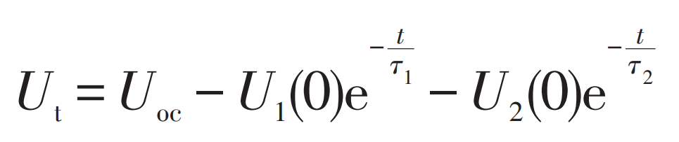
The circuit diagram of the second-order RC equivalent circuit model is shown in Figure 1. The model consists of two RC resistive and capacitive networks: the first RC resistive and capacitive network describes the impedance during electrode to electrode transmission, while R1 and C1 represent the activation polarization internal resistance and activation polarization capacitance, respectively; The second RC resistance capacitance network describes the impedance of lithium ion diffusion in the electrode material, with R2 and C2 representing the concentration polarization internal resistance and concentration polarization capacitance, respectively. U1 and U2 represent the terminal voltages of two RC resistive and capacitive networks, respectively; Uoc represents the open circuit voltage (OCV) of the battery, which is a non-linear function corresponding to the SOC of the battery; R0 represents the Ohmic internal resistance of the battery. I is the terminal current of the battery, which is specified to be positive in the direction of discharge current; Ut represents the terminal voltage of the battery.
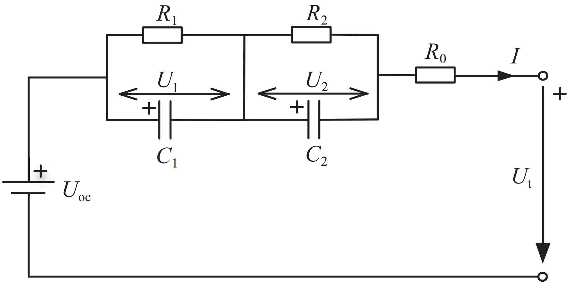
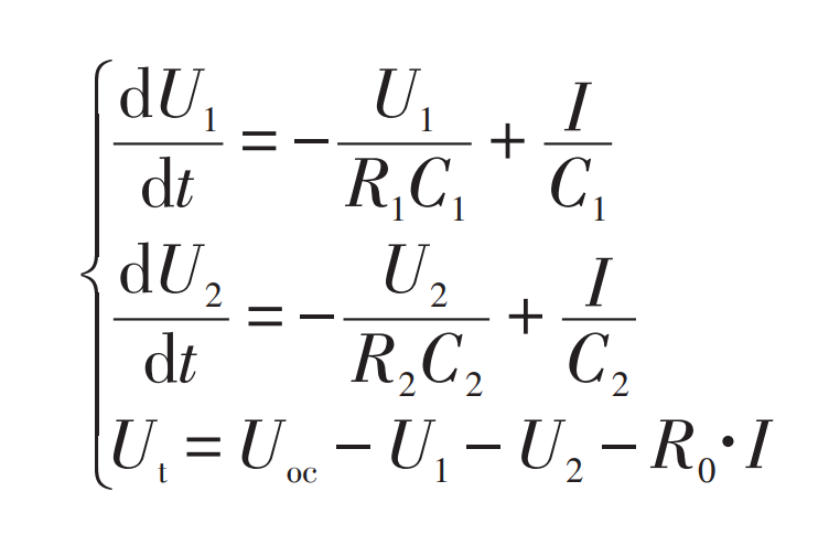
According to Figure 1, the following relationship can be obtained from Kirchhoff’s law of voltage and current:
1.2 Parameter Identification
The parameters to be identified in the model include Uoc, R1, C1, R2, C2, and R0. Open circuit voltage experiments and cyclic pulse discharge experiments were used to identify the model parameters. Considering that the model parameters of the battery are functions of three factors: SOC, temperature, and current ratio, and the accuracy of the model is easily affected by these factors. In order to improve the accuracy of the basic model and avoid the traditional offline modeling methods from deepening the aging degree of retired batteries, this paper only considers the influence of SOC on the model parameters during parameter identification experiments. Then, the model is compensated for using the model terminal voltage error at different temperatures and current multiples, further improving the accuracy of the basic model. The experimental object of the battery used is a 18650 type lithium cobalt oxide battery, with a nominal voltage of 362 V, a maximum voltage of 4.2 V, a cut-off voltage of 2.75 V, and a nominal capacity of 2.15 Ah.
1.2.1 Identification of open circuit voltage
The calibration experimental steps for the relationship curve between open circuit voltage and SOC are as follows:
1) At room temperature, the battery is charged to full capacity using a standard charging method of constant current followed by constant voltage. After standing for 2 hours, the open circuit voltage value is measured and recorded, and the SOC corresponding to this voltage value is calibrated to 1.
2) Discharge at a constant current rate of 1.0C (the current at which the battery is fully discharged for 1 hour) for 6 minutes, that is, release 10% of the capacity and let it stand for 2 hours. Record the open circuit voltage value at this time, and calibrate the corresponding SOC to 0.9.
3) Repeat step 2) until the SOC drops to 0 or the battery terminal voltage drops to 2.75 V, and stop the experiment.
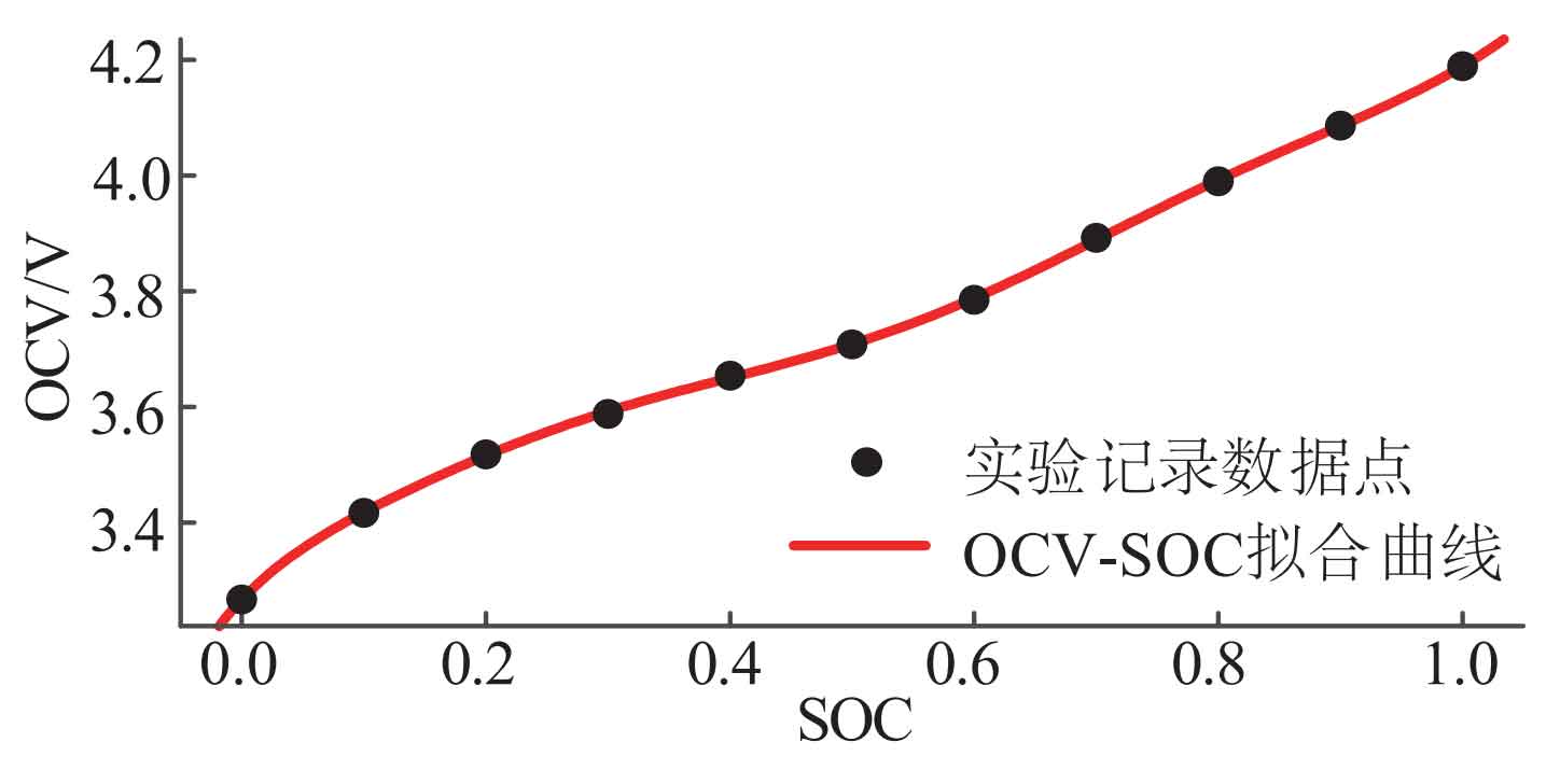
Using Matlab’s Cftool toolbox to perform curve fitting on experimental data, taking into account the computational complexity and fitting accuracy, an 8-order polynomial function was selected as the fitting result, and the relationship equation and curve of OCV-SOC were obtained as shown in Equation (2) and Figure 2, respectively.
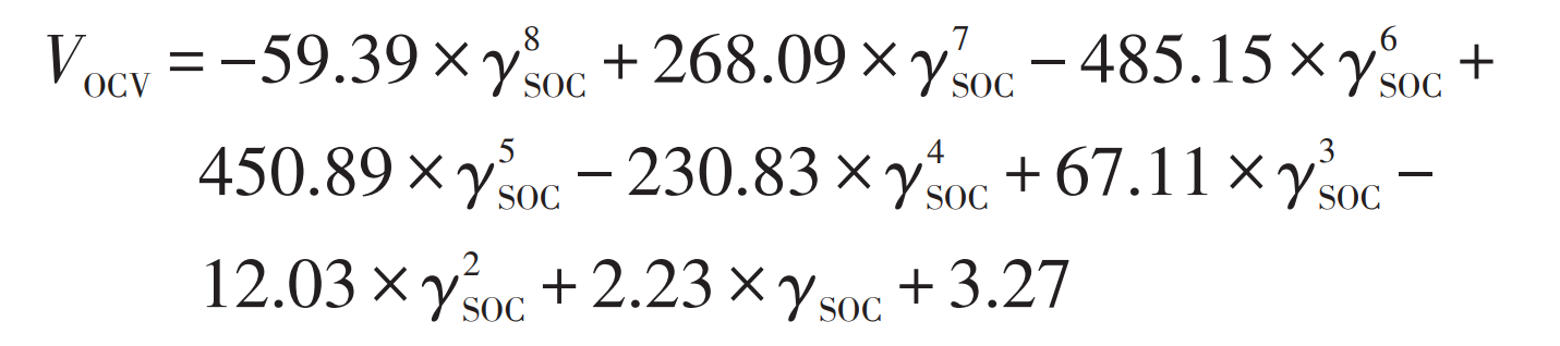
In the formula: VOCV – OCV value; γ SOC – SOC value.
1.2.2 Identification of resistance and capacitance parameters
For the parameters R1, C1, R2, C2, and R0 in the battery model, this paper adopts cyclic pulse discharge experiments for identification. By utilizing the voltage and current values that can be measured externally, the complex characteristic changes inside the battery can be demonstrated. The specific experimental steps are as follows:
1) Charge the battery to full charge and let it stand for 2 hours at room temperature using a standard charging method of constant current followed by constant voltage.
2) Discharge at a constant current rate of 1.0C for 3 minutes, that is, release 5% of the capacity and let it stand for 5 minutes. Record the changes in battery terminal voltage throughout the entire process.
3) Repeat step 2) until the SOC drops to 0 or the battery terminal voltage drops to 2.75 V, and stop the experiment.
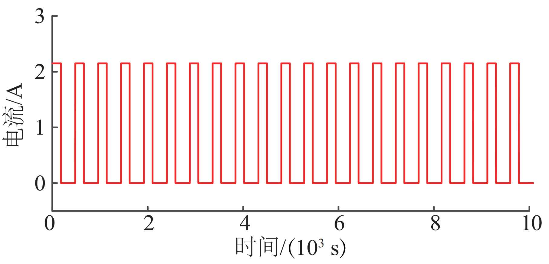
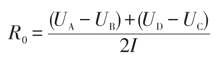
Figure 3 shows the current variation curve of the cyclic pulse discharge experiment. Figure 4 shows the terminal voltage response curve within one pulse cycle in step 2), which can be divided into four stages: in the first stage, the AB segment, where the battery undergoes a jumping decrease in terminal voltage from standing to sudden current discharge. For the second-order RC equivalent circuit model, the voltage on capacitors C1 and C2 cannot jump abruptly, so the jump voltage is mainly determined by the ohmic internal resistance R0. In the second stage BC segment, as the discharge time increases, the battery terminal voltage decreases exponentially due to the influence of two RC resistive and capacitive networks. In the CD segment of the third stage and the DE segment of the fourth stage, the battery changes from loaded discharge to unloaded rest, and the voltage response also undergoes a process of jumping up and exponential characteristic rising. The principle is the same as in the AB and BC segments.
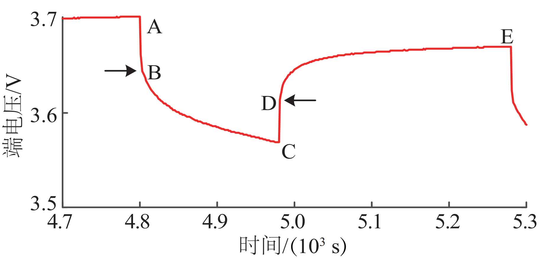
Taking Figure 4 as an example, the specific derivation process for identifying the resistance and capacitance parameters in a pulse cycle is presented below. The AB and CD segments in the figure exhibit strong internal resistance characteristics, so the average pressure difference between these two segments can be selected to calculate the Ohmic internal resistance. The calculation formula is:
The BC and DE segments are both the results of the RC resistance capacitance network, and the values of the polarization resistance and capacitance can be obtained by exponentially fitting these two curves.
The DE stage is the zero input response stage where the RC network loses excitation after removing the pulse current. Taking point D as the time t=0, the zero input response expressions of the two RC networks are:
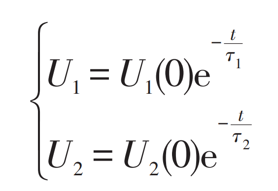
In the equation: τ 1 and τ 2- Time constant of two RC resistive capacitance networks. At this point, the terminal voltage output equation of the battery is shown in equation (5). By using Matlab’s Cftool toolbox to fit the DE segment curve, two time constants can be obtained τ 1 and τ The value of 2.
The BC segment is the response process of loading and discharging after a period of quiescence. At this time, the voltage at both ends of C1 and C2 is approximately 0, so the BC segment can be regarded as the zero state response stage of the RC network. Taking point B as the time t=0, the zero state response expressions of the two RC networks are:
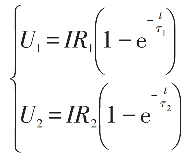
At this point, the terminal voltage output equation of the battery is:
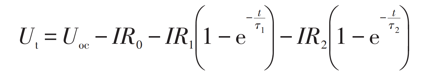
Substituting the two time constants obtained from the DE segment into equation (7) and fitting them with Matlab exponent, the values of R1 and R2 can be obtained. Based on τ 1=R1C1, τ 2=R2C2, the values of C1 and C2 can be obtained.
After fitting the voltage curves of all pulse cycles according to the above steps, a dynamic model can be obtained to simulate the complex electrochemical reaction process inside the battery when the SOC changes.
2.Error analysis and improvement of battery model
2.1 Model error analysis at different temperatures and discharge rates
Based on the battery model established above that only introduces the influence factor of SOC, the model error of this model at different temperatures and discharge rates will be analyzed below. According to the operating temperature range of the selected battery object in this article, constant current discharge experiments were conducted at rates of 0.3C, 0.5C, 1.0C, and 1.2C under constant temperature conditions of -10, 0, 25, and 30 ℃, and the terminal voltage change data of the battery was recorded. The specific experimental steps are:
1) Charge the battery to full charge and let it stand for 2 hours at room temperature using a standard charging method of constant current followed by constant voltage.
2) Place the fully charged battery in a set temperature incubator and let it sit for more than 30 minutes.
3) Under different temperature conditions, perform constant current discharge on the battery at different discharge rates until the battery terminal voltage drops to 2.75 V, and stop the experiment. Record the changes in the battery terminal voltage throughout the entire process.
Using the Lookup Table module of Matlab/Simulink, the identified model parameters are imported into the simulation model, and the current is used as the input of the model. The output terminal voltage of the model is compared with the measured terminal voltage under the same excitation current. The comparison waveform between the model terminal voltage and the measured terminal voltage at different temperatures and discharge rates is shown in Figure 5.
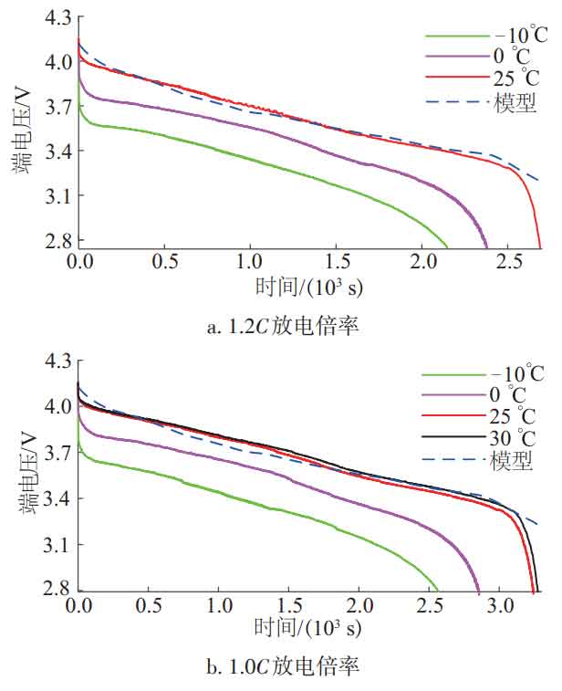
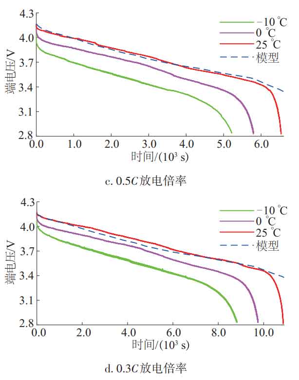
From Figure 5, it can be seen that when the discharge rate is the same, the lower the temperature, the greater the model error; When the temperature is the same, the larger the discharge rate, the greater the model error. This indicates that the second-order RC equivalent circuit model that only considers the influence of SOC still has a certain simulation error compared to real batteries.
By processing the terminal voltage error data under different operating conditions, the model error table shown in Table 1 is obtained, where the definitions of two errors are shown in Equation (8).
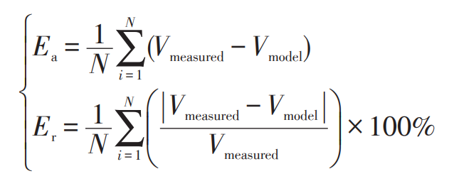
In the formula: Ea – average error; Er – average relative error; Vmeasured – measured terminal voltage value; Vmodel – The voltage value at the output end of the model.
From Table 1, it can be seen that under the same temperature conditions, the model error is basically positively correlated with the discharge rate; Under the same discharge rate conditions, the model error is negatively correlated with temperature, and the data in the table is consistent with the conclusion drawn in Figure 5. The reason for the analysis is that as the discharge rate increases, the chemical reactions inside the battery become more intense, especially in the late stage of discharge. The internal reactions are more complex and variable, and the model parameters are fitted based on a fixed current rate. At this time, the description effect of the model on the battery will decrease. At the same time, the model parameters are also fitted based on room temperature conditions. As the temperature decreases, the temperature difference with room temperature increases, which also leads to a deterioration in the model’s description of the battery.
| Temperature/℃ | Discharge rate/C | Mean error/V | Average relative error/% |
| -10 | 0.3 | -0.30448 | 8.96398 |
| -10 | 0.5 | -0.35606 | 10.64951 |
| -10 | 1.0 | -0.39037 | 11.98736 |
| -10 | 1.2 | -0.38877 | 12.00907 |
| 0 | 0.3 | -0.13635 | 3.92416 |
| 0 | 0.5 | -0.16265 | 4.73560 |
| 0 | 1.0 | -0.19331 | 5.75616 |
| 0 | 1.2 | -0.20025 | 5.98380 |
| 25 | 0.3 | -0.00528 | 0.89725 |
| 25 | 0.5 | -0.01439 | 0.91627 |
| 25 | 1.0 | -0.01201 | 1.13460 |
| 25 | 1.2 | -0.01115 | 0.87952 |
| 30 | 1.0 | 0.01126 | 0.97636 |
It is worth noting that under constant temperature conditions of 30 ℃, this article only provides the model error for constant current discharge at a rate of 1.0C. This design method lays the foundation for the construction and analysis of the BP neural network in the following text.
2.2 Construction and Analysis of BP Neural Networks Based on Few Samples
Through the above analysis, the average error of the model is affected by temperature and load current changes, which is equivalent to a controlled voltage source. Therefore, this voltage source can be compensated into the circuit model to improve model accuracy. However, in order to obtain model errors under a wide range of temperature and current conditions, repeating the experimental process described above for retired batteries will not only consume a lot of time, but also cause a loss of battery cycle life, thereby reducing the cascade utilization rate of retired batteries.
Based on the above issues, a method is proposed to expand the prediction of large sample data with small sample data. Firstly, the average error data of the model under existing temperature and discharge rate conditions is fitted as an expression, and then a BP neural network is trained based on the expression. The neural network is used to predict the average error of the model under wide range temperature and current conditions, and it is compensated into the circuit model to improve the accuracy of the model.
By using Matlab’s Cftool toolbox to fit the temperature, load current, and average error data in Table 1, various order expressions of model error can be obtained. The corresponding output values of each expression at different discharge rates and temperatures are shown in Table 2. Among them, the independent variable x represents temperature, and the independent variable y represents load current.
| Temperature/℃ | Discharge rate/C | Mean error/V | f(x^3,y^3)/V | f(x^3,y^2)/V | f(x^3,y^1)/V | f(x^2,y^3)/V | f(x^2,y^2)/V | f(x^2,y^1)/V | f(x^1,y^3)/V | f(x^1,y^2)/V | f(x^1,y^1)/V |
| -10 | 0.3 | -0.30448 | -0.3079 | -0.3096 | -0.3205 | -0.3058 | -0.3108 | -0.3160 | -0.2707 | -0.2715 | -0.2942 |
| -10 | 0.5 | -0.35606 | -0.3517 | -0.3489 | -0.3380 | -0.3538 | -0.3390 | -0.3345 | -0.3070 | -0.3065 | -0.3056 |
| -10 | 1.0 | -0.39037 | -0.3897 | -0.3928 | -0.3819 | -0.3867 | -0.3854 | -0.3807 | -0.3508 | -0.3502 | -0.3338 |
| -10 | 1.2 | -0.38877 | -0.3900 | -0.3885 | -0.3994 | -0.3876 | -0.3942 | -0.3992 | -0.3492 | -0.3501 | -0.3452 |
| 0 | 0.3 | -0.13635 | -0.1323 | -0.1340 | -0.1422 | -0.1323 | -0.1444 | -0.1486 | -0.1894 | -0.1897 | -0.2031 |
| 0 | 0.5 | -0.16265 | -0.1671 | -0.1642 | -0.1560 | -0.1700 | -0.1669 | -0.1614 | -0.2208 | -0.2207 | -0.2144 |
| 0 | 1.0 | -0.19331 | -0.1955 | -0.1985 | -0.1903 | -0.1976 | -0.1989 | -0.1935 | -0.2545 | -0.2542 | -0.2427 |
| 0 | 1.2 | -0.20025 | -0.1974 | -0.1958 | -0.2041 | -0.2046 | -0.2020 | -0.2063 | -0.2498 | -0.2501 | -0.2540 |
| 25 | 0.3 | -0.00528 | -0.0058 | -0.0073 | -0.0089 | -0.0080 | -0.0011 | -0.0062 | 0.0141 | 0.0148 | 0.0248 |
| 25 | 0.5 | -0.01439 | -0.0142 | -0.0112 | -0.0097 | -0.0094 | -0.0093 | -0.0049 | -0.0052 | -0.0061 | 0.0135 |
| 25 | 1.0 | -0.01201 | -0.0102 | -0.0131 | -0.0116 | 0.0029 | -0.0053 | -0.0016 | -0.0138 | -0.0144 | -0.0148 |
| 25 | 1.2 | -0.01115 | -0.0125 | -0.0108 | -0.0124 | -0.0084 | 0.0060 | -0.0003 | -0.0011 | -0.0002 | -0.0261 |
| 30 | 1.0 | 0.01126 | 0.0113 | 0.0110 | 0.0110 | -0.0037 | -0.0134 | -0.0106 | 0.0344 | 0.0336 | 0.0308 |
By comparing the output values of various order expressions, it can be observed that when x and y are both 3rd order, the expression has the smallest difference between its output value and the average error of the model compared to the other order expressions in Table 2, and the expression is:
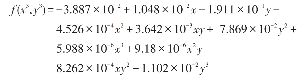
Based on equation (9), train the BP neural network with 1 input layer, 2 nodes, and input values of load current and temperature; The hidden layer is 1 layer, with 5 nodes; The output layer is 1 layer, with 1 node and an output of (f x3, y3).
The training set of the BP neural network consists of the changing current and temperature, as well as the corresponding model average error. The current starts at 0.6 A and increases by an amplitude of 0.05 A to 2.6 A; The temperature starts at -10 ℃ and increases by 1 ℃ to 30 ℃. Set the transfer function of the hidden layer to tansig, the transfer function of the output layer to purelin, and the training function to Levenberg_ The trainlm of the Marquardt algorithm.
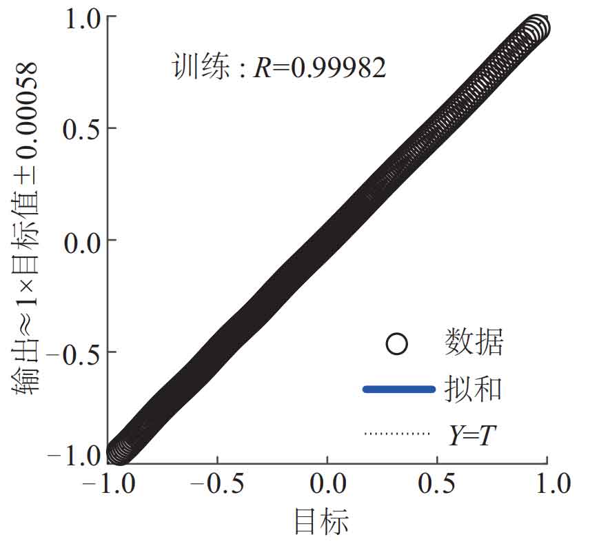
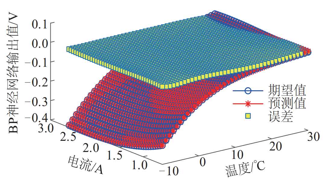
Figure 6 shows the regression curve of the BP neural network, with R=0.9982, which is close to GF. Figure 7 shows the comparison curve and error curve between the predicted and expected values of the BP neural network, where the x-axis represents temperature, the y-axis represents load current, and the z-axis represents the average error of the model output by the BP neural network. It can be seen that the predicted value and expected value almost completely coincide, and the error is basically zero.
| Temperature/℃ | Discharge rate/C | Mean error/V | (f x ^ 3, y ^ 3) Output value/V | BP neural network output value/V |
| -10 | 0.3 | -0.30448 | -0.3079 | -0.3063 |
| -10 | 0.5 | -0.35606 | -0.3517 | -0.3507 |
| -10 | 1.0 | -0.39037 | -0.3897 | -0.3880 |
| -10 | 1.2 | -0.38877 | -0.3900 | -0.3910 |
| 0 | 0.3 | -0.13635 | -0.1323 | -0.1331 |
| 0 | 0.5 | -0.16265 | -0.1671 | -0.1660 |
| 0 | 1.0 | -0.19331 | -0.1955 | -0.1948 |
| 0 | 1.2 | -0.20025 | -0.1974 | -0.1974 |
| 25 | 0.3 | -0.00528 | -0.0058 | -0.0054 |
| 25 | 0.5 | -0.01439 | -0.0142 | -0.0136 |
| 25 | 1.0 | -0.01201 | -0.0102 | -0.0099 |
| 25 | 1.2 | -0.01115 | -0.0125 | -0.0109 |
| 30 | 1.0 | 0.01126 | 0.0113 | 0.0109 |
Table 3 shows the model error values of BP neural network training. From the data in the table, it can be seen that the output values of the BP neural network are basically equal to the output values of the expression. This once again validates the conclusion drawn in Figure 7, indicating that the BP neural network has achieved the expected effect.
To verify the better voltage compensation effect of the BP neural network compared to various order expressions, the operating conditions of the battery were set at different charging and discharging rates and temperatures. The output values of the BP neural network and the output values of each order expression were compared, as shown in Tables 4 and 5.
| Temperature/℃ | Discharge rate/C | Mean error/V | BP neural network output value/V | f(x^3,y^3)/V | f(x^3,y^2)/V | f(x^3,y^1)/V | f(x^2,y^3)/V | f(x^2,y^2)/V | f(x^2,y^1)/V | f(x^1,y^3)/V | f(x^1,y^2)/V | f(x^1,y^1)/V |
| 5 | 1.0 | -0.12937 | -0.1327 | -0.1331 | -0.1367 | -0.1298 | -0.1264 | -0.1290 | -0.1235 | -0.2064 | -0.2063 | -0.1971 |
| 20 | 1.0 | -0.04662 | -0.0306 | -0.0309 | -0.0351 | -0.0322 | -0.0061 | -0.0129 | -0.0084 | -0.0619 | -0.0624 | -0.0604 |
| 25 | 0.7 | -0.0124 | -0.0134 | -0.0142 | -0.0132 | -0.0104 | -0.0029 | -0.0119 | -0.3807 | -0.0155 | -0.0169 | 0.0022 |
| 25 | 2.5 | 0.08079 | 0.0193 | -0.5077 | 0.0467 | -0.0174 | -1.0054 | 0.2146 | 0.0081 | 0.3132 | 0.3368 | -0.0997 |
| 25 | 4.0 | 0.17874 | 0.0646 | -3.4943 | 0.2048 | -0.0232 | -6.3973 | 0.7468 | 0.0179 | 1.2009 | 1.2520 | -0.1846 |
| 40 | 0.5 | 0.02911 | 0.0252 | 0.0454 | 0.0613 | 0.0579 | -0.1179 | -0.1017 | -0.1004 | 0.1241 | 0.1227 | 0.1502 |
| 40 | 1.0 | 0.06293 | 0.0651 | 0.0748 | 0.0848 | 0.0813 | -0.0634 | -0.0762 | -0.0759 | 0.1306 | 0.1295 | 0.1220 |
Table 4 shows the model error table corresponding to the BP neural network and various order expressions under different temperatures and discharge rates. The data in the table can be analyzed from the following three aspects:
| Temperature/℃ | Discharge rate/C | Mean error/V | BP neural network output value/V | f(x^3,y^3)/V | f(x^3,y^2)/V | f(x^3,y^1)/V | f(x^2,y^3)/V | f(x^2,y^2)/V | f(x^2,y^1)/V | f(x^1,y^3)/V | f(x^1,y^2)/V | f(x^1,y^1)/V |
| 25 | 0.6 | 0.09083 | 0.0912 | 0.2639 | 0.0303 | -0.0055 | 0.3105 | 0.1009 | -0.0119 | 0.2038 | 0.2263 | 0.0747 |
| 25 | 1.0 | 0.07606 | 0.1176 | 0.6144 | 0.0601 | -0.0039 | 0.7860 | 0.1871 | -0.0146 | 0.3521 | 0.3950 | 0.0984 |
1) The discharge rate and temperature within the BP neural network training set were validated under three operating conditions: a discharge rate of 1C at a temperature of 5 ℃, a discharge rate of 1.0C at a temperature of 20 ℃, and a discharge rate of 0.7C at a temperature of 25 ℃. It can be observed that the output value of the BP neural network is basically equal to the output value of the expressions (fx3, y3), indicating once again that the BP neural network has achieved the expected effect.
2) The set temperature is 25 ℃, and the discharge rate is 2.5C and 4.0C, respectively, to verify the discharge rate outside the BP neural network training set. It can be found that when the discharge rate exceeds the range of the training set, the output value of the BP neural network has a smaller difference from the average error of the model compared to the expressions (fx3, y3), indicating that the BP neural network has better predictive performance.
3) The set temperature is 40 ℃, and the discharge rate is 0.5C and 1.0C, respectively, to verify the temperature outside the BP neural network training set. It can be found that even if the error data of only 1.0C discharge rate is fitted at a temperature of 30 ℃, the BP neural network can still make accurate predictions of the model error when discharging at 0.5C rate under constant temperature conditions of 40 ℃, and the prediction effect is better than that of the expression. This verifies the feasibility of the constructed BP neural network, which is also consistent with the data in Table 1.
Table 5 shows the model error tables corresponding to BP neural network and various order expressions under different charging rates. The temperature was set at 25 ℃, and the model error was verified at 0.6C and 1.0C charging rates. It can also be found that the output value of the BP neural network during charging has better predictive performance compared to the expressions (fx3, y3), once again verifying the feasibility of the constructed BP neural network.
By analyzing the data in Tables 4 and 5, the following conclusions can be drawn:
1) The neural network trained under small range temperature and small discharge rate conditions can accurately predict model errors outside the range temperature and under large discharge rate conditions;
2) The neural network trained under small range discharge rate conditions can also make good predictions of model errors under charging rate conditions. Although the output value of the neural network is slightly worse than other expressions of different orders under certain operating conditions, overall, the BP neural network has better predictive and adaptability than expressions of different orders, indicating the feasibility of the proposed method for expanding small sample data.
2.3 Model Error Analysis with BP Neural Network Compensation
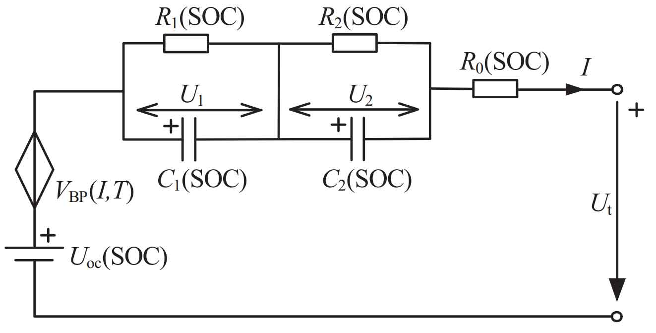
Connect the controlled voltage source generated by the BP neural network in series into the second-order RC equivalent circuit model to achieve dynamic compensation for the terminal voltage of the battery model. The second-order RC equivalent circuit model with an additional controlled voltage source is shown in Figure 8, where VBP (I, T) is the controlled voltage source, influenced by two independent variables: current and temperature.
| Temperature/℃ | Discharge rate/C | Average error before improvement/V | Improved average error/V | Average relative error before improvement/% | Average relative error after improvement/% |
| -10 | 0.3 | -0.30448 | 0.00182 | 8.96398 | 2.00785 |
| -10 | 0.5 | -0.35606 | -0.00176 | 10.64951 | 1.77452 |
| -10 | 1.0 | -0.39037 | -0.00237 | 11.98736 | 1.88532 |
| -10 | 1.2 | -0.38877 | 0.00223 | 12.00907 | 1.90318 |
| 0 | 0.3 | -0.13635 | -0.00325 | 3.92461 | 1.60652 |
| 0 | 0.5 | -0.16265 | 0.00335 | 4.73560 | 1.87115 |
| 0 | 1.0 | -0.19331 | 0.00149 | 5.75616 | 2.07222 |
| 0 | 1.2 | -0.20025 | -0.00285 | 5.98380 | 1.94170 |
| 25 | 0.3 | -0.00528 | 0.00012 | 0.89725 | 0.80045 |
| 25 | 0.5 | -0.01439 | -0.00079 | 0.91627 | 0.87531 |
| 25 | 1.0 | -0.01201 | -0.00211 | 1.13460 | 1.09101 |
| 25 | 1.2 | -0.01115 | -0.00025 | 0.87952 | 0.82777 |
| 30 | 1.0 | 0.01126 | 0.00036 | 0.97636 | 0.93394 |
To verify the accuracy of the improved model, the improved model terminal voltage in Figure 5 was compared with the measured terminal voltage under different operating conditions. Taking the 1.2C discharge rate as an example, the waveform of terminal voltage comparison before and after model improvement at different temperatures is shown in Figure 9.
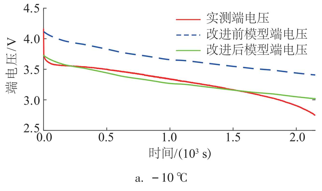
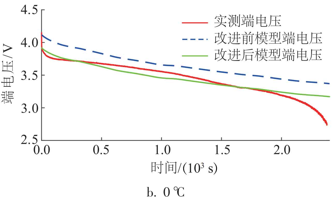
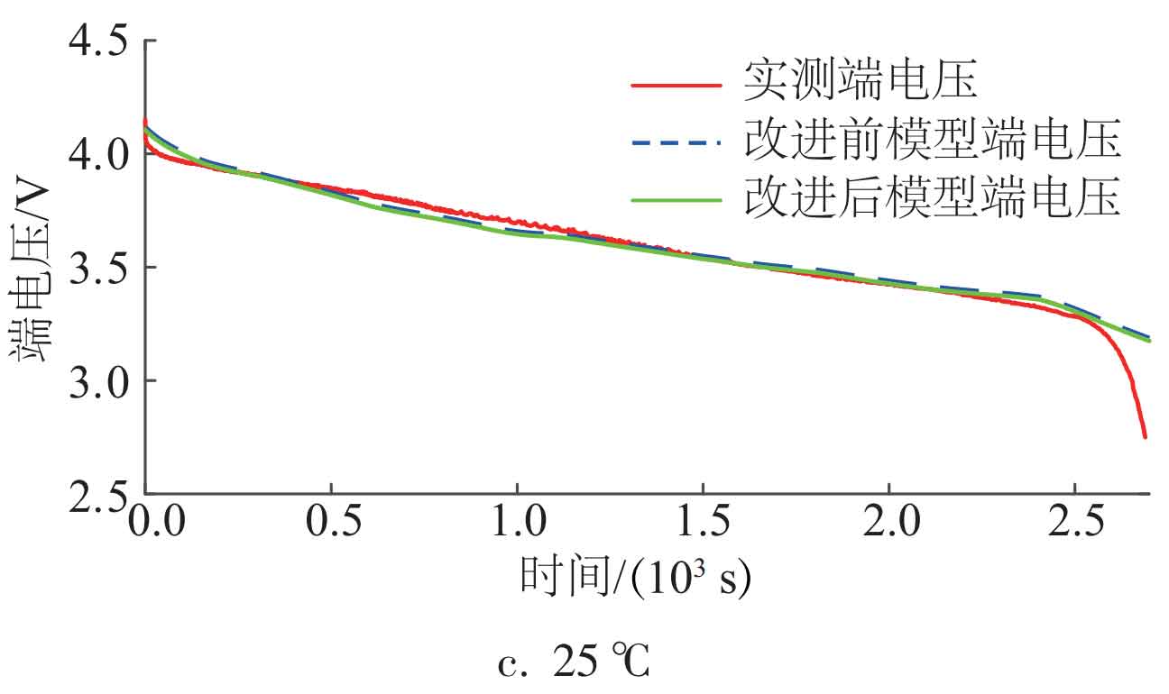
From Figure 9, it can be seen that under different temperature operating conditions, the improved model terminal voltage curve is closer to the measured terminal voltage curve and has smaller terminal voltage error, indicating that the model accuracy has been significantly improved after adding BP neural network compensation. The error comparison before and after model improvement is shown in Table 6. From the data in Table 6, it can be seen that the average error value and average relative error value of the improved model have been significantly reduced, indicating that the adaptability of the improved model has been improved under different temperatures and current ratios, and the simulation effect on batteries is better.
3.Application of model-based energy storage system
The model proposed in this article can be used to uniformly simplify and sort the battery cells in the energy storage system, forming an energy storage system for new energy generation. At the same time, based on the model, the prediction and analysis of battery cell heating and the application of battery thermal management can be carried out, which is beneficial for the safety evaluation of energy storage systems. Based on this model, the battery terminal voltage and battery SOC of the energy storage system can be predicted, which can be used to evaluate the operational energy efficiency simulation of the energy storage system.
4. Conclusion
Based on the second-order RC equivalent circuit model, a model improvement method with an additional controlled voltage source is proposed. The effectiveness of the proposed method and the improved model was verified through theoretical analysis and experimental results, and the following main conclusions were obtained:
1) The BP neural network has better predictive performance than expressions, and the proposed method of expanding the prediction of large sample data with small sample data has certain feasibility and practical application value in engineering.
2) The improved model’s terminal voltage curve can better follow the actual measured battery terminal voltage curve, and the simulation effect of the battery is better at different temperatures and current multiples, resulting in improved model accuracy.
3) This model can be used for sorting hierarchical batteries and monitoring and evaluating the operational status of energy storage systems, which can promote the application of lithium-ion batteries in new energy generation and energy storage systems.