
Solar energy has become one of the most promising renewable energy sources in the context of global energy transformation. Photovoltaic (PV) panels, also known as solar panels, convert sunlight directly into electricity through the photovoltaic effect. The efficiency of this conversion strongly depends on the surface condition of the panels. Accumulated dust, cracks, breakage, hot spots, and other defects can significantly reduce the output power and even pose safety risks. Therefore, reliable and automated defect detection for solar panels is of great practical importance.
In this work, I address two major pain points in conventional manual inspection of solar panels: long inspection time and low precision. I propose a deep-learning-based rapid inspection framework designed for unmanned aerial vehicle (UAV) imagery. The framework integrates image enhancement, feature extraction, and an improved YOLOv4 model enhanced with a selective kernel network (SKNet) attention mechanism. The main contributions are threefold. First, I develop an image preprocessing pipeline that corrects lens distortion and removes haze to improve image quality under adverse conditions. Second, I propose a fusion of shape and texture features to better distinguish true defects from dust and stains, which often look similar in color and geometry. Third, I introduce SKNet into different parts of the YOLOv4 architecture and systematically evaluate the optimal insertion position. The experimental results show that embedding SKNet into the backbone network improves the detection mAP@0.5 by 2.3%, and the improved model exhibits higher confidence for small defect targets.
The remainder of this article is organized as follows. Section 2 reviews the fundamentals of convolutional neural networks and object detection frameworks. Section 3 presents the image preprocessing and feature extraction methods. Section 4 describes the improved YOLOv4 model, dataset preparation, experiments, and performance analysis. Section 5 concludes the work and discusses future research directions.
1. Introduction
1.1 Background and Motivation
The global energy landscape is undergoing a profound transformation due to environmental concerns, climate change, and the depletion of fossil fuels. Renewable energy, especially solar photovoltaic power, plays a pivotal role in this transition. According to recent statistics, China added 48.2 GW of PV capacity in 2020, a 60% increase compared to 2019, bringing the total installed capacity to 253 GW. The PV power generation in 2020 reached 260.5 TWh, accounting for 3.5% of the total electricity generation. Governments worldwide have implemented supportive policies to promote the adoption of solar energy, and the trend is expected to continue.
Solar panels are typically installed outdoors, either on rooftops or in large ground-mounted power plants. During their long service life, they are exposed to various environmental stresses, including wind, sand, hail, temperature fluctuation, and human activities. These stresses lead to different types of defects, such as cracks, broken busbars, hot spots, delamination, snail trails, and foreign object adhesion. Any defect can reduce the photoelectric conversion efficiency and, in severe cases, cause short circuits or fire hazards. For example, micro-cracks in silicon solar cells can create localized shunts, leading to hot spots and accelerated degradation. Research has shown that a single crack located between busbars can decrease the output power by up to 60% when both ends are fractured. Therefore, timely and accurate detection of defects is critical to maintain the reliability and profitability of PV systems.
Traditional manual inspection methods rely on visual inspection by trained workers, sometimes with the aid of thermal cameras or digital multimeters. However, these methods are time-consuming, labor-intensive, and often miss small or subtle defects. In large-scale PV plants, the sheer number of panels makes manual inspection impractical on a regular basis. Drones equipped with high-resolution cameras can cover large areas quickly, but the resulting images still require automatic analysis to be useful. This motivates the development of intelligent defect detection systems based on deep learning.
1.2 Related Work
Several approaches have been proposed for PV panel defect detection. They can be broadly categorized into three groups: gradient-based methods, clustering-based methods, and machine-learning-based methods.
1.2.1 Gradient-Based Methods
Gradient-based methods exploit the intensity difference at the boundary between a defective area and a normal area. Anwar and Abdullah proposed an improved anisotropic diffusion filter combined with gradient information to sharpen defects while smoothing background noise. Tsai et al. combined gradient features with mean shift clustering to detect panel edges, automatically finding cluster numbers without manual estimation. Lai introduced a particle swarm optimization (PSO) algorithm with gradient features to detect defects, reporting robustness for noisy images.
1.2.2 Clustering-Based Methods
Clustering-based methods partition the image into defective and non-defective regions using algorithms such as K-means or Otsu thresholding. Xu and Fu used the Otsu method after filtering and semantic segmentation to isolate individual panels, then applied Hough transform to detect linear features and compare with the reference image. Liu et al. employed L0 gradient minimization followed by K-means clustering for fabric defect detection. Li used entropy rate clustering with superpixels to extract defect regions. These methods often require manual parameter tuning and may fail when defects are not well separated from the background in the color space.
1.2.3 Machine-Learning-Based Methods
With the advent of deep learning, object detection algorithms based on convolutional neural networks (CNNs) have achieved remarkable success in various industrial inspection tasks. Silva et al. applied support vector machines (SVM) with local descriptors for panel defect classification. Li et al. designed a lightweight cascaded CNN for surface defect detection. Liu et al. used generative adversarial networks (GANs) with independent component analysis for thermographic defect detection. MobileNet-SSD and other lightweight architectures have also been explored. However, these methods often suffer from a trade-off between speed and accuracy, especially for small defects that occupy only a few pixels.
A comparison of these methods is provided in Table 1.
| Category | Principle | Advantages | Disadvantages |
|---|---|---|---|
| Gradient-based | Uses intensity variation at defect boundaries | Simple, effective for high-contrast defects | Sensitive to noise; requires clear edge |
| Clustering-based | Segments image into defect/background regions | Handles various defect types | Manual parameter selection; not fully automatic |
| Machine learning | Learns features from labeled samples | High accuracy, real-time potential | Needs large dataset; may miss unseen defects |
1.3 Contributions
The main contributions of this work are summarized as follows:
- A complete UAV image based PV panel defect detection pipeline is proposed, from image acquisition to defect localization.
- An image enhancement module is designed to correct geometric distortion and remove haze, improving the quality of input images for subsequent analysis.
- A feature extraction scheme merging shape descriptors and texture descriptors is introduced to reduce false positives caused by the color similarity between defects and dust.
- An improved YOLOv4 model with the SKNet attention mechanism is proposed. The optimal insertion position of SKNet is investigated through systematic experiments.
2. Fundamentals of Deep Learning
2.1 Convolutional Neural Networks
Convolutional neural networks (CNNs) have become the mainstream approach for image recognition tasks since the breakthrough of AlexNet in 2012. A CNN automatically learns hierarchical feature representations from raw pixels, eliminating the need for hand-crafted features. The basic building blocks of a CNN include convolutional layers, activation functions, pooling layers, and fully connected layers.
2.1.1 Basic Units
An artificial neuron computes a weighted sum of its inputs, adds a bias, and passes the result through a nonlinear activation function. The output \(y\) can be expressed as:
\[
y = f\left( \sum_{i=1}^{n} w_i x_i + b \right)
\]
where \(x_i\) are the input signals, \(w_i\) are the weights, \(b\) is the bias, and \(f\) is an activation function. Common activation functions include ReLU, sigmoid, and tanh. ReLU is defined as \(f(x)=\max(0,x)\) and is widely used because it accelerates convergence and alleviates the vanishing gradient problem.
2.1.2 Convolutional Layer
The convolution operation applies a set of learnable kernels to the input feature map. For a 2D image \(I\) and a kernel \(K\), the convolution output is:
\[
(I * K)(i,j) = \sum_{m}\sum_{n} I(i+m, j+n) K(m,n)
\]
Convolution preserves spatial relationships and shares parameters, drastically reducing the number of parameters compared to fully connected layers.
2.1.3 Pooling Layer
Pooling down-samples the feature map to reduce computational complexity and increase translation invariance. The two common types are max pooling and average pooling. For a pooling window of size \(p \times p\) with stride \(s\), the output size is approximately \(W/p\) if \(s=p\). Pooling helps the network focus on higher-level features.
2.1.4 Fully Connected Layer
The fully connected layer maps the learned distributed features to the final classification scores. It is typically placed at the end of the network. For a binary classification problem, the output can be passed through a sigmoid function to obtain a probability.
2.2 Traditional Object Detection
Before the deep learning era, object detection relied on hand-crafted features and classical classifiers. The Viola-Jones method achieved real-time face detection using Haar-like features and an AdaBoost cascade. Histogram of Oriented Gradients (HOG) descriptors were popular for pedestrian detection. Deformable Part Models (DPM) extended HOG by considering deformable parts and achieved state-of-the-art results at the time. These methods often required careful feature engineering and struggled with variations in scale, orientation, and illumination.
2.3 Modern Object Detection Models
Modern detection models fall into two categories: two-stage detectors and one-stage detectors.
2.3.1 Two-Stage Detectors
Two-stage detectors first generate region proposals and then classify each proposal. The R-CNN series is representative. R-CNN extracts around 2000 region proposals using selective search, warps them to a fixed size, extracts features with a CNN, and classifies with an SVM. However, R-CNN is slow due to repeated feature extraction. SPP-Net introduced spatial pyramid pooling to avoid cropping and warping, allowing variable input sizes. Fast R-CNN improved speed by using a single feature extraction pass and multi-task loss. Faster R-CNN replaced selective search with a Region Proposal Network (RPN), enabling end-to-end training. These detectors achieve high accuracy but are generally slower than one-stage detectors.
2.3.2 One-Stage Detectors
One-stage detectors directly predict object categories and bounding boxes without a separate proposal stage. The YOLO (You Only Look Once) family is the most prominent. YOLO divides the image into a grid and each grid cell predicts bounding boxes and class probabilities. YOLOv2 introduced batch normalization, anchor boxes, dimension priors, and a Darknet-19 backbone. YOLOv3 used a deeper Darknet-53 with residual connections and multi-scale feature maps via a feature pyramid network (FPN). YOLOv4 further improved by incorporating CSPDarknet, SPP, PANet, and numerous training tricks. One-stage detectors are typically faster and are well-suited for real-time applications.
Given the need for real-time processing of UAV images while maintaining high accuracy for small defects, I choose YOLOv4 as the baseline model and propose to enhance it with a selective kernel attention mechanism.
3. Image Processing and Feature Extraction for Solar Panels
3.1 Image Preprocessing
Images captured by UAVs often suffer from degradation due to camera shake, haze, and lens distortion. These degradations can reduce the accuracy of defect detection. Therefore, preprocessing is essential to improve image quality before feeding the images into the detection model.
3.1.1 Distortion Correction
Camera lenses introduce geometric distortion, mainly radial and tangential distortion. Radial distortion causes straight lines to appear curved; it can be barrel or pincushion distortion. Tangential distortion arises from misalignment of the lens assembly. A widely used distortion model, introduced by Brown, can be expressed as:
\[
x_{\text{corrected}} = x(1 + k_1 r^2 + k_2 r^4 + k_3 r^6) + 2 p_1 x y + p_2 (r^2 + 2 x^2)
\]
\[
y_{\text{corrected}} = y(1 + k_1 r^2 + k_2 r^4 + k_3 r^6) + p_1 (r^2 + 2 y^2) + 2 p_2 x y
\]
where \((x,y)\) are the original distorted pixel coordinates, \(r\) is the radial distance from the principal point, \(k_i\) are radial distortion coefficients, and \(p_i\) are tangential distortion coefficients. In this work, I apply a self-calibration method using a bundle adjustment with additional parameters in aerial triangulation. The corrected coordinates are obtained by iteratively estimating the distortion parameters.
The simulation results show that the corrected images have significantly improved geometric accuracy, allowing later feature extraction to be more reliable.
3.1.2 Haze Removal
Haze reduces visibility and contrast, which seriously affects the performance of visual inspection algorithms. For dehazing, I adopt the dark channel prior method proposed by He et al. The dark channel of an image is defined as:
\[
J^{\text{dark}}(x) = \min_{c \in \{R,G,B\}} \left( \min_{y \in \Omega(x)} J^c(y) \right)
\]
For a clear outdoor image, the dark channel tends to be extremely low, close to zero. The haze imaging model is:
\[
I(x) = J(x) t(x) + A (1 – t(x))
\]
where \(I\) is the observed hazy image, \(J\) is the scene radiance to be recovered, \(A\) is the global atmospheric light, and \(t\) is the transmission map. Estimating the transmission: using the dark channel prior, the transmission can be estimated as:
\[
\tilde{t}(x) = 1 – \min_{c} \left( \min_{y \in \Omega(x)} \frac{I^c(y)}{A^c} \right)
\]
After obtaining the transmission map, the scene radiance is recovered by:
\[
J(x) = \frac{I(x) – A}{\max(t(x), t_0)} + A
\]
In practice, the atmospheric light is estimated by selecting the top 0.1% brightest pixels in the dark channel and then taking the maximum intensity among them. The simulation results demonstrate that the dehazed image has much better visual contrast and detail, which helps the subsequent detection network distinguish defects from the background.
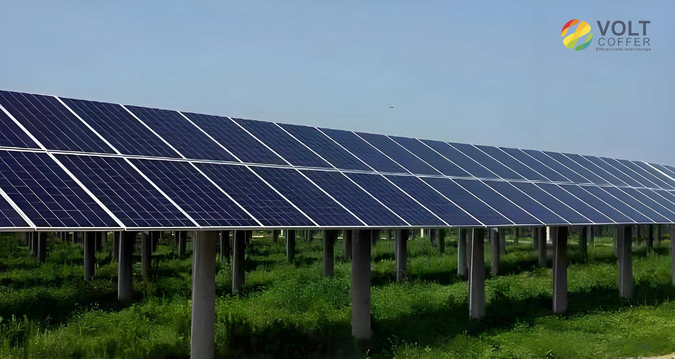
An example of a photovoltaic panel with improved visibility after preprocessing is shown below.
3.2 Feature Extraction for Solar Panel Defects
3.2.1 Color Features
Color is an intuitive visual feature. Since defects such as cracks and hot spots often have a darker color than the surrounding normal area, color features can help localize them. Common color representations include color histograms, color moments, and color coherence vectors. Color moments provide a compact representation: the first three moments (mean, variance, skewness) for each color channel. For a color channel, the mean \(\mu\), variance \(\sigma^2\), and skewness \(s\) are defined as:
\[
\mu = \frac{1}{N} \sum_{j=1}^{N} p_j
\]
\[
\sigma^2 = \frac{1}{N} \sum_{j=1}^{N} (p_j – \mu)^2
\]
\[
s = \frac{1}{N} \sum_{j=1}^{N} (p_j – \mu)^3
\]
These moments are robust to changes in illumination and viewpoint but may not capture spatial layout.
3.2.2 Texture Features
Texture describes the spatial arrangement of pixel intensities. It is a global feature and is relatively robust to noise. For solar panel defects, texture can distinguish the regular pattern of solar cells from irregular defect patterns. I consider several texture descriptors:
- Gray Level Difference Statistics: compute the gray value difference between a pixel and its neighbor. The difference \(\Delta g = g(x,y) – g(x+\Delta x, y+\Delta y)\) is used to form histograms. The mean, contrast, and entropy of these histograms characterize texture roughness.
- Autocorrelation Function: measures the similarity between the image and its shifted version; the roughness of the texture can be inferred from the decay rate of the autocorrelation.
- Gray Level Co-occurrence Matrix (GLCM): captures joint probabilities of pixel pairs at specific offsets. From GLCM, one can derive contrast, energy, entropy, homogeneity, and correlation.
In the final implementation, I use a Gabor filter for texture feature extraction because it mimics the human visual system and is effective in capturing directional texture patterns. A 2D Gabor filter is given by:
\[
G(x,y;\lambda,\theta,\psi,\sigma,\gamma) = \exp\left(-\frac{x’^2 + \gamma^2 y’^2}{2\sigma^2}\right) \cos\left(2\pi \frac{x’}{\lambda} + \psi\right)
\]
where \(x’ = x\cos\theta + y\sin\theta\), \(y’ = -x\sin\theta + y\cos\theta\), \(\lambda\) is the wavelength, \(\theta\) is the orientation, \(\psi\) is the phase offset, \(\sigma\) is the standard deviation, and \(\gamma\) is the spatial aspect ratio. The texture feature is constructed by filtering the image with multiple Gabor filters at different orientations and frequencies, then extracting the local energy.
3.2.3 Shape Features
Shape features are important for recognizing defects with distinct contours. Two common approaches are the Fourier shape descriptor and moment invariants. The Fourier descriptor starts by representing the boundary as a complex sequence \(s(k) = x(k) + j y(k)\). The discrete Fourier transform is:
\[
a(u) = \sum_{k=0}^{N-1} s(k) e^{-j 2\pi u k / N}
\]
The boundary can be reconstructed using the inverse transform. Moment invariants, such as Hu moments, are derived from normalized central moments and are invariant to translation, scaling, and rotation. They are useful when the defect has a consistent shape but appears in different orientations.
3.2.4 Fusion of Texture and Shape Features
Defects on solar panels often have a shape and color similar to dust or stains, leading to false positives when only one type of feature is used. For example, a dark spot could be either a crack or a piece of dust. To reduce misclassification, I propose to concatenate shape features (Fourier descriptor) and texture features (Gabor-based) into a unified feature vector. The fusion can be written as:
\[
\mathbf{F} = [\alpha \mathbf{F}_{\text{shape}}^T, \beta \mathbf{F}_{\text{texture}}^T]^T
\]
where \(\mathbf{F}_{\text{shape}}\) and \(\mathbf{F}_{\text{texture}}\) are the feature vectors and \(\alpha\), \(\beta\) are normalization weights. After fusion, the feature vector is used in a classifier or directly learned by a CNN.
Simulation results show that the fused feature extraction makes the local defect features more pronounced than using a single feature extraction method. The fused features help the detection model distinguish true defects from visually similar non-defective objects.
4. Solar Panel Defect Detection
4.1 Dataset Preparation
I used a public dataset of solar panel defect images from Baidu AI Studio. The dataset contains images of solar cells with various defects such as cracks, broken grids, and dust. Since the focus is on defect detection, I manually annotated 728 images using the LabelImg tool. The annotations were grouped into two classes: “defect” and “dust”. Defects include cracks, breakage, hot spots, etc.; dust represents foreign particles or stains that are not true panel defects but should ideally be distinguished from defects. Bounding boxes were placed around each target, and the annotations were saved as XML files in the VOC format. Table 2 shows a few examples of the annotation information.
| filename | width | height | class | xmin | ymin | xmax | ymax |
|---|---|---|---|---|---|---|---|
| Cel0001.png | 300 | 300 | defect | 64 | 114 | 84 | 192 |
| Cel0001.png | 300 | 300 | dust | 144 | 82 | 154 | 96 |
The XML files are parsed into a CSV table containing the filename, image size, class, and coordinates. The dataset is then randomly split into training and test sets with a ratio of 9:1. Data augmentation is performed on-the-fly, including random horizontal flips, brightness changes, and scale jitter, to improve generalization.
4.2 Improved YOLOv4 Model
4.2.1 Review of YOLOv4
YOLOv4 is a state-of-the-art one-stage detector that builds upon YOLOv3. Its backbone is CSPDarknet53, which combines a CSPNet structure with Darknet53 to reduce computational redundancy while maintaining rich gradient information. The neck employs a PANet (Path Aggregation Network) that fuses features from different scales, and an SPP (Spatial Pyramid Pooling) module to enlarge the receptive field. The head is similar to YOLOv3, consisting of three detection branches at scales of 19×19, 38×38, and 76×76. The loss function includes CIoU loss for bounding box regression, binary cross-entropy for objectness, and categorical cross-entropy for classification. YOLOv4 also uses Mish activation, Mosaic data augmentation, and other tricks.
The output feature maps have a shape of \(S \times S \times (3 \times (C+5))\), where \(S\) is the grid size, \(3\) is the number of anchor boxes per grid cell, \(C\) is the number of classes, and \(5\) accounts for the four box offsets and one objectness score.
4.2.2 SKNet Attention Mechanism
Selective Kernel Networks (SKNet) is an attention mechanism that adaptively selects the size of the convolution kernel based on the input. It comprises three operations: Split, Fuse, and Select. In the Split stage, the input is convolved with multiple kernels of different sizes. In the Fuse stage, the resulting feature maps are summed and passed through a global average pooling to generate channel-wise statistics. The fused descriptor \(s\) is obtained by:
\[
s_c = \frac{1}{H \times W} \sum_{i=1}^{H} \sum_{j=1}^{W} U_c(i,j)
\]
A fully connected layer generates a compact feature \(z\):
\[
z = \delta(W_2 \sigma(W_1 s))
\]
where \(\delta\) is ReLU and \(\sigma\) is a linear transform. In the Select stage, a softmax operation assigns weights to each kernel. For two branches, the weights are:
\[
a_c = \frac{e^{z_c^1}}{e^{z_c^1} + e^{z_c^2}}, \quad b_c = 1 – a_c
\]
The final feature map is the weighted sum:
\[
V_c = a_c \cdot U_c^1 + b_c \cdot U_c^2
\]
This mechanism enables the network to dynamically choose the appropriate receptive field for each spatial location, which is beneficial for detecting defects with varying sizes and shapes.
4.2.3 Integration of SKNet into YOLOv4
To determine where SKNet should be inserted for maximum benefit, I designed three variants:
- YOLOv4-SKnet-A: SKNet is inserted into the backbone network, right after each concat layer in the CSP modules and after the add layer in the ResUnit modules.
- YOLOv4-SKnet-B: SKNet is placed in the neck (PANet) after each concat layer that fuses features from different scales.
- YOLOv4-SKnet-C: SKNet is placed before the detection heads, applying the attention to the final feature maps.
The structural modification is inspired by the observation that small objects rely on fine-grained features from middle and low layers. Inserting an attention module in the backbone may help the network focus on informative channels and kernels at an early stage.
4.3 Experimental Setup
The experiments were conducted on a workstation with an Intel Xeon Silver 4110 CPU and an NVIDIA GeForce RTX 2080 Ti GPU with 11 GB memory. The software environment included Windows 10, Python 3.7, and PyTorch 1.2.0. The input image size was set to 416×416. The initial learning rate was 0.001, decayed by a factor of 0.1 every 50 epochs. Momentum was 0.9, weight decay was 0.0005, and the stochastic gradient descent (SGD) optimizer with a batch size of 8 was used. The model was trained for 200 epochs.
4.4 Performance Metrics
Four metrics were used to evaluate the detection performance: precision (P), recall (R), F1 score, and mean average precision (mAP). They are defined as:
\[
P = \frac{TP}{TP+FP}
\]
\[
R = \frac{TP}{TP+FN}
\]
\[
F1 = \frac{2 P R}{P+R}
\]
\[
mAP = \frac{1}{C} \sum_{i=1}^{C} AP_i
\]
where \(TP\) is the number of true positives, \(FP\) is the number of false positives, \(FN\) is the number of false negatives, \(C\) is the number of classes, and \(AP\) is the area under the precision-recall curve. mAP@0.5 indicates that the IoU threshold is 0.5.
4.5 Results and Analysis
Table 3 reports the performance of the baseline YOLOv4 and the three improved variants on the test set.
| Model | P (%) | R (%) | mAP@0.5 (%) |
|---|---|---|---|
| YOLOv4 | 60.2 | 72.4 | 71.2 |
| YOLOv4-SKNet-A | 57.2 | 74.5 | 73.5 |
| YOLOv4-SKNet-B | 59.5 | 71.3 | 69.4 |
| YOLOv4-SKNet-C | 52.4 | 76.2 | 70.3 |
From the results, it is clear that inserting SKNet into the backbone (YOLOv4-SKNet-A) improves the mAP by 2.3% compared to the baseline. In contrast, inserting SKNet into the neck (B) or head (C) does not bring gains; in fact, the mAP slightly drops. This suggests that the backbone layer already contains rich mid- and low-level features that are crucial for detecting small targets. Applying attention at this stage allows the network to adaptively select the most relevant convolutional kernels, enhancing the representation of defect regions. The recall value for variant A (74.5%) is also higher than that of the baseline (72.4%), indicating that more true defects are successfully discovered. The precision is slightly lower, which may be due to a small increase in false positives; however, the overall mAP improvement shows that the trade-off is acceptable.
To visually verify the improvement, I compared the detection results before and after the modification. The improved model yields higher confidence scores for small defects and successfully detects some instances that the baseline misses, particularly for the “dust” class. This demonstrates that the SKNet attention module in the backbone helps the model focus on subtle but discriminative features.
The loss curves during training also indicate that YOLOv4-SKNet-A converges stably and achieves a lower final loss than the baseline, confirming the effectiveness of the attention mechanism.
5. Conclusion and Future Work
5.1 Summary
In this article, I presented a comprehensive study on defect detection of solar panels based on deep learning. The work was motivated by the practical need for efficient and accurate inspection of photovoltaic systems. I first reviewed the background and existing methods, highlighting the limitations of manual inspection and conventional image processing. Then I introduced an image enhancement pipeline that corrects lens distortion and removes haze from UAV images, improving the visual quality and the performance of the subsequent detection model.
For feature extraction, I proposed a fusion of shape and texture features, which helps distinguish true defects from dust and stains. The feature fusion method was tested and showed better discriminative ability than using a single feature type.
The core of the work is an improved YOLOv4 model integrated with the SKNet attention mechanism. Through systematic experiments, I found that inserting SKNet into the backbone network is the most effective configuration. The improved model achieved a mAP@0.5 of 73.5%, which is 2.3% higher than the baseline YOLOv4. The detection confidence for small defects was significantly improved, and the model could detect targets that were previously missed.
5.2 Future Work
There are several directions to extend this research. First, the proposed pipeline has been validated on a relatively small dataset; collecting a larger and more diverse dataset with various panel types and defect conditions would enhance generalization. Second, other attention mechanisms, such as CBAM or channel-wise attention, could be compared to SKNet for this task. Third, more advanced network architectures, including transformer-based detectors, might offer further accuracy improvements. Fourth, the deployment of the model on embedded devices such as drones or edge computers should be explored to realize real-time on-board detection. Finally, the integration of thermal imaging with visible-light images could provide complementary information and improve the detection of hot spots and internal defects.
In conclusion, the proposed deep-learning-based defect detection technology for solar panels demonstrates great potential to reduce maintenance costs, improve power generation efficiency, and ensure the safe operation of photovoltaic systems. I hope that this work contributes to the growing field of automated PV inspection and inspires further innovations in the application of deep learning to renewable energy infrastructure.