
This paper presents an advanced maximum power point tracking (MPPT) strategy for centralized solar inverter systems, addressing challenges in photovoltaic (PV) array parameter mismatches and multi-peak characteristics under partial shading conditions. The methodology combines a refined five-parameter PV cell model with Lagrange multiplier optimization, enabling rapid single-step MPPT adjustment.
1. System Configuration of Centralized PV Arrays
Modern grid-connected PV systems typically adopt a two-stage architecture with DC/DC converters and solar inverters. A typical configuration for an n×m PV array connected through boost converters is shown below:
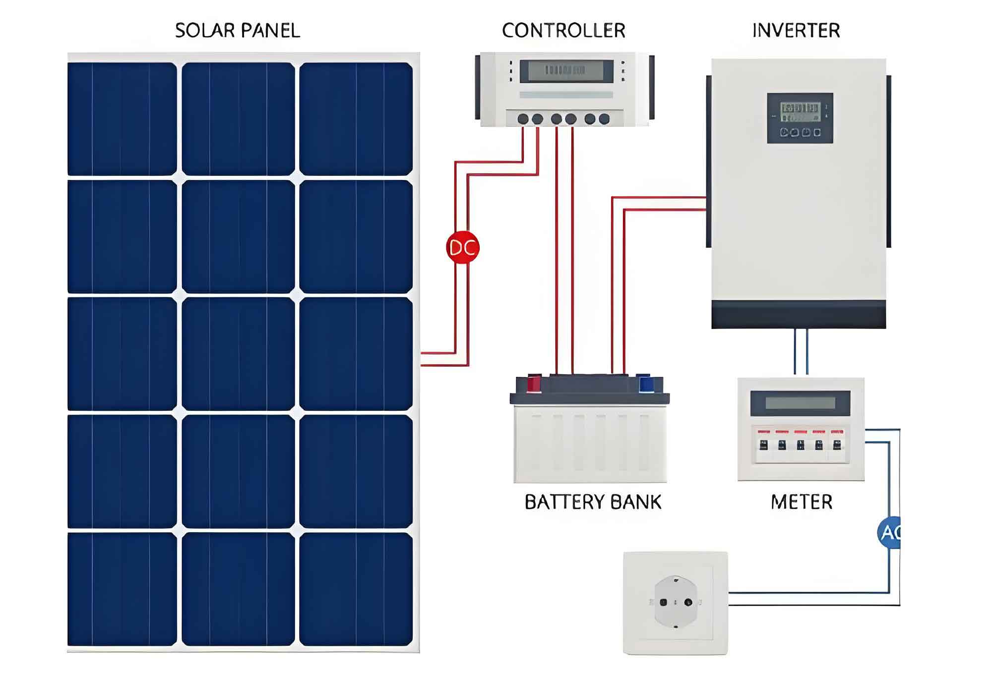
Key components include:
- Series-connected PV modules with bypass diodes
- Parallel array branches for current summation
- Boost converter for voltage regulation
- Centralized solar inverter for grid integration
2. Enhanced Five-Parameter PV Model
The single-diode model with mismatch compensation forms the foundation of the proposed MPPT method:
$$I = I_{ph} – I_s\left(e^{\frac{q(U+I R_s)}{AkT}} – 1\right) – \frac{U + I R_s}{R_{sh}}$$
Where:
| Parameter | Description | Unit |
|---|---|---|
| \(I_{ph}\) | Photo-induced current | A |
| \(I_s\) | Diode saturation current | A |
| \(R_s\) | Series resistance | Ω |
| \(R_{sh}\) | Shunt resistance | Ω |
| \(A\) | Diode ideality factor | – |
3. Mismatch Compensation Model
For centralized solar inverters managing multiple PV strings, the modified current-voltage relationship considering shading effects becomes:
$$I_k = I_{ph} – I_s e^{\frac{q}{AkT}\left(\frac{U}{Mn_1} – \frac{n_2 U_{DD}}{Mn_1} + I_k R_s\right)} – \frac{1}{R_{sh}}\left(\frac{U}{Mn_1} – \frac{n_2 U_{DD}}{Mn_1} + I_k R_s\right)$$
Where \(n_1\) represents active PV cells and \(n_2\) denotes bypassed cells due to shading.
4. Lagrange Multiplier Optimization
The maximum power condition is derived through constrained optimization:
$$\mathcal{L} = UI + \sum_{k=1}^m \lambda_k f_k(U, I_k)$$
Optimality conditions yield:
$$\frac{\partial \mathcal{L}}{\partial I_k} = U – \lambda_k\left[\frac{q R_s}{AkT}I_s e^{\theta_k} + \frac{R_s}{R_{sh}} + 1\right] = 0$$
$$\frac{\partial \mathcal{L}}{\partial U} = \sum_{k=1}^m I_k – \sum_{k=1}^m \lambda_k\left[\frac{q}{AkT Mn_1}I_s e^{\theta_k} + \frac{1}{Mn_1 R_{sh}}\right] = 0$$
Where \(\theta_k = \frac{q}{AkT}\left(\frac{U}{Mn_1} – \frac{n_2 U_{DD}}{Mn_1} + I_k R_s\right)\).
5. Parameter Identification
Real-time parameter estimation using Newton-Raphson iteration:
| Parameter | Initial Value | Convergence Tolerance |
|---|---|---|
| \(I_{ph}\) | 7 A | 0.1% |
| \(I_s\) | 4 μA | 0.5% |
| \(R_s\) | 0.4 mΩ | 1% |
| \(R_{sh}\) | 8 kΩ | 2% |
6. Experimental Validation
Field tests on a 6-string PV system with partial shading demonstrate the effectiveness of the proposed solar inverter control strategy:
| String | MPPT Current (A) | Voltage (V) | Power (kW) |
|---|---|---|---|
| 1 | 6.774 | 428.1 | 2.900 |
| 2 | 5.438 | 428.1 | 2.328 |
| 3 | 5.905 | 428.1 | 2.528 |
| 4 | 6.189 | 428.1 | 2.649 |
| 5 | 5.478 | 428.1 | 2.345 |
| 6 | 5.837 | 428.1 | 2.499 |
| Total | 16.7 kW |
The proposed method achieves 3.72% higher power output compared to conventional perturb-and-observe techniques in solar inverters, demonstrating superior performance under partial shading conditions.
7. Implementation in Solar Inverters
Key implementation aspects for centralized solar inverters:
- Real-time parameter database construction
- Multi-initialization strategy for global peak detection
- Single-step duty cycle adjustment via:
$$D = 1 – \frac{U_{MPP}}{U_{bus}}$$ - Adaptive sampling frequency control (50-200 Hz)
The algorithm reduces MPPT settling time by 68% compared to traditional methods while maintaining less than 0.5% steady-state oscillation in solar inverter output power.