
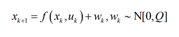
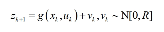
Batteries have complex chemical reactions inside them during operation and are influenced by various non battery factors, making them a nonlinear system. The EKF method can linearize nonlinear systems, so it can be used to solve the nonlinear problem of the charging and discharging processes of lithium-ion batteries. However, the accuracy of EKF is affected by various parameters. This section uses deep reinforcement learning to optimize and improve EKF. By effectively verifying the charging state estimation algorithm for lithium-ion batteries, the EKF algorithm can be quickly adjusted and achieve higher accuracy.
1. Prediction of State of Charge Based on EKF
1.1 EKF principle
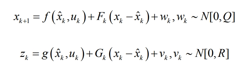
Under the condition of linear Gaussian, KF can achieve dynamic estimation of the target, but the estimation effect of this method can only be guaranteed in linear systems. However, EKF can overcome the shortcomings of the former by expanding the coefficient matrix of the equation using Taylor series, and ignoring or approximating higher-order terms of quadratic or higher order. Due to the non-linear charging and discharging process of lithium-ion batteries, EKF can be used to solve this nonlinear problem. Since the system processed by EKF is discrete, the basic electrical equations of the second-order RC equivalent circuit model will also be discretized to form state and observation equations, which will be substituted into the EKF system, namely:
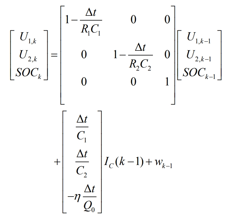
Among them, Δ T is the sampling time, K is the Coulombic efficiency, Q0 is the rated capacity of the battery, wk is the system noise, and kv is the observation noise.
The following are the basic steps for extending Kalman filtering:
(1) Linearization
The state equation and observation equation are:
Place f (xk, uk,) and g (xk, uk) at xk=x ˆ By linearizing around k and ignoring higher-order terms above second order, we obtain:
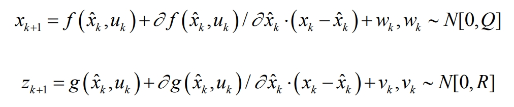
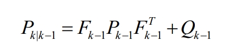
Take Fk=(x ˆ K, uk)/ σ X ˆ K and Gk= σ X (x ˆ K, uk)/ σ X ˆ k. The state equation and observation equation can be transformed into:
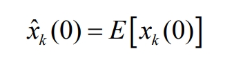
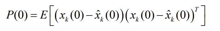
(2) Initialize
If k=0, the initial state value is:
The initial error covariance difference is:
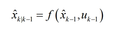
(3) Time and status updates
The forward status value is:
The forward error covariance is:
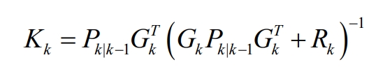
The Kalman filter gain is:
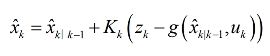
Update the state vector for the next moment to:
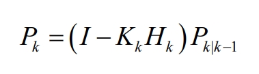
Update the error covariance at the next moment as:
(4) Repeat cycle steps (1) – (3)
1.2 SOC prediction based on EKF
When conducting simulation verification of the algorithm, it is necessary to set the initial values of the parameters inside the algorithm. In the simulation section of this article, the initial value of the state vector is set to x (0)=[0.900], and the third-order unit matrix is used as the initial value of the error covariance. During the simulation, the process noise covariance matrix and measurement noise covariance matrix can be adjusted based on the simulation estimation effect.
2. State of Charge Estimation for EKF Optimization Based on Double DQN
2.1 MDP model
Reinforcement learning is a multi-layer algorithm that simulates the implicit distribution of data. Taking feedback on the environment as input to the system, its continuous decisions are adaptive to the environment. Its main feature is not annotating the data. Its main idea is to continuously interact with the environment through intelligent agents, conduct trial and error based on feedback information such as errors, and record learning, thereby optimizing decision-making actions accordingly. The purpose is to find the optimal strategy or maximum reward. The interaction between the aforementioned intelligent agent. The basic principle is to learn based on (positive/negative) rewards. If a specific action in the system brings positive rewards in the environment, it is highly likely that the trend towards this action in the future will strengthen. Otherwise, the system generated action will be weakened.
Reinforcement learning has Markov characteristics, so from a mathematical perspective, it is a Markov Decision Process (MDP). By seeking the optimal strategy, the overall return function expectation in the decision-making process can reach the optimal expectation. MDP is usually represented as (S, A, P, R), where S is the state space, A is the control action, P is the transition probability between states, and R is the reward function.
The equivalent circuit model and extended Kalman filter of lithium-ion batteries are considered as the environment, and the Double DQN algorithm based on lithium battery energy storage prediction is used as the intelligent agent. Therefore, the MDP model for battery energy storage prediction.
Its target task is to change the parameters of EKF to improve the accuracy of SOC estimation for lithium-ion batteries. The specified requirements for its target parameters are as follows:
(1) State space
The state space in the Markov decision process includes the current and next new states. In order to achieve high simulation verification results, it is necessary to select appropriate and appropriate number of state parameters.
(2) Action Space
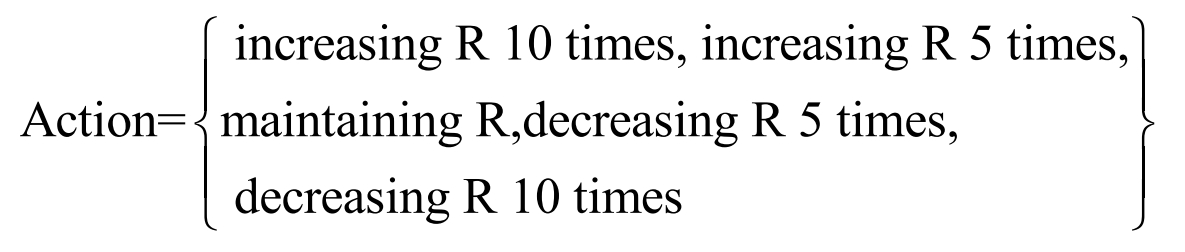
The intelligent agent in the MDP model for energy storage prediction makes control actions based on state and real-time rewards, thereby continuously improving the accuracy of the state of charge. Therefore, the action space needs to select parameters that can improve the accuracy of EKF estimation.
(3) State transition probability
It depends on the actual state of the environment after executing the action.
(4) Instant rewards
Represents the reward obtained by performing an action in the current state and transferring to the new state at the next time. The purpose of the MDP model for predicting lithium battery energy storage is to obtain maximum rewards. Therefore, the setting of immediate rewards requires that relevant information reflecting the accuracy of the state of charge can be obtained through observation.
2.2 DQN
Q-learning is a technology for optimizing control, mainly based on multiple updates of value functions and dynamic learning mechanisms, used to solve Markov decision problems. A series of actions, observations, and rewards are all included in this algorithm, with the core being to maximize the expected total reward, that is, to examine the action value function under strategy S, using Q^ τ (s, a) represents.
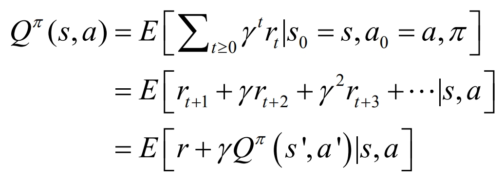
Where s represents the state; S’ represents the state after the action of s; A represents the state; The strategy represents the strategy that transitions from the current state π (st, at) to the next action at; E represents the cumulative expectation under strategy π; γ∈ (0,1) is the discount factor.
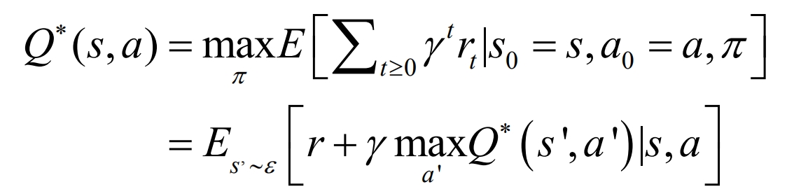
It is difficult to maximize the expected total return in the initial steps, that is, to obtain the optimal value of the action value function, and the optimal Q value needs to be used, defined as:
Based on the above theoretical framework, the Q-Learning algorithm is an MDP model for predicting the energy storage of lithium-ion batteries, which can store and estimate the value functions of various states. That is, it can update all states and actions of the iteration. In the process of continuous interaction between the RL controller and the control area, the process of action evaluation is to update the iterative value function using equations.

Among them, α∈ (0,1) is the learning rate, which is positively correlated with the convergence speed of the algorithm. Max is the maximum value of the selected Q function.
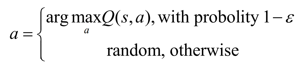
After the iteration gradually converges, the optimal strategy is π * (s, a) to select the action with the highest Q value in state s, which is the greedy strategy (H − greedy). This process is called action selection, which is:
In the practical work of lithium-ion batteries, the state and action space generated by the energy storage prediction system of lithium-ion batteries may have a relatively large scale, so an optimized Q-learning algorithm may cause the problem of “curse of dimensionality”. To solve this problem, it is necessary to achieve complementary advantages between reinforcement learning and deep learning, thus forming deep reinforcement learning. Using deep learning to solve strategies or value functions, the objective function is optimized using backpropagation.
DeepMind has produced two versions of Deep Q Network (DQN). Among them, the 2013 version is the initial version. This algorithm combines Q-learning, experience regeneration mechanism [83], and convolutional neural network-based techniques to generate the target Q-value. It is used to input the state of the intelligent agent, output the corresponding Q value for each action, and obtain the state of the action to be executed.
This algorithm combines deep learning and reinforcement learning using objective function, objective network, and experience playback mechanism, which can effectively learn the value function of reinforcement learning tasks and provide action strategies for intelligent agents. By using a dual network structure, the 2015 DQN version added a target network, reducing the correlation between the current Q value and the target Q value, and significantly improving the stability of the DQN algorithm.
2.3 Double DQN
DQN uses a greedy strategy when updating Q values and selecting actions, and only has one neural network. Therefore, the Q value is often overestimated. In other words, the estimated Q value is greater than the actual Q value. An improved version of DQN – Double DQN – has been proposed to address the above issues. It uses two Q-networks to solve the overestimation problem generated by the learning process algorithm.
Double DQN utilizes the current Q network Q (st, at, θ) Responsible for the selection of actions and the target Q network Q ‘(st, at, θ’) Responsible for calculating the target Q value and reducing the overestimation problem of the value function caused by the calculation deviation of max Q value, as shown in the following equation:
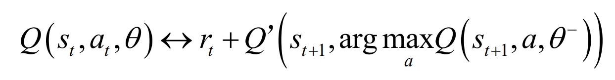
Among them, is the parameter of the current Q network and is the parameter of the target Q network. If the Q value overestimates a, select it. So the Q ‘value will provide an appropriate value. If the Q ‘value is overestimated, then the Q’ value will not select an action.
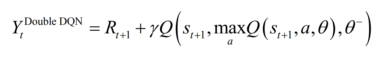
The target Q value based on Double DQN is calculated as follows:
The Double DQN algorithm is as follows:
(Parameters: Maximum value of experience trajectory M, number of iterations T, maximum value of stored samples N, action a, probability of greedy strategy, current network Q, target network Q ‘, experience replay size n, target network Q’ parameter update frequency C)
(1) Initialize experience pool D, store the maximum value of experience samples as N, the current Q network and parameter T
(2) Initialize target network Q ‘and parameters θ ‘ , Make θ’=θ
(3) Repeat experience trajectory, from 1 to M
(4) Repeat the single experience trajectory from t=1 to t=T
(5) Select action at based on H − degree
(6) Execute action at to receive reward rt
(7) Update status s (t+1)=st
(8) Store experience samples (st, at, rt, st+1) into experience pool D
(9) Randomly sampling small batches of stored samples from experience pool D
(10) Repeat from i=1 to i=n
(11) Set the target Q value to Yi
(12) Calculate the loss function (Yi Q (si, ai, θ))^ Parameters in 2 θ , Update target network Q
(13) Reset every C steps θ- = θ, Update target network
For the MDP model for predicting lithium-ion battery energy storage in this article, the Double DQN algorithm uses a greedy strategy to select the action at, the agent receives an immediate reward rt, the environment updates the state s (t+1), and the experience replay pool stores the experience samples (st, at, rt, st+1) generated during the state transition process. Every C steps, the controller randomly extracts a small batch of data from it and performs experience playback to update the network parameters, thereby storing the data of the reward function and improving the convergence of the network model. At the beginning of the iteration, the Double DQN algorithm is in a learning state and all parameters are in an unstable state. As the number of iterations increases, the neural network parameters gradually converge, and the actions output by the controller gradually increase the reward function.
2.4 EKF Algorithm for Lithium Battery SOC Estimation Based on Double DQN Optimization
The dynamic situation of executing control actions is used to optimize control training and continuously optimize EKF parameters throughout the entire learning process. The balance between exploration and utilization can be achieved through greedy strategies( ε- Policy. Thus, it ensures the convergence speed of the algorithm while avoiding learning falling into local optimization. The Double DQN module minimizes the loss function by optimizing the objective function for each iteration (Yi Q (si, ai, θ))^ 2.
The operation process of lithium-ion battery SOC estimation based on the entire Double DQN and EKF consists of two parts, namely environment and intelligent agent.
The first part is the environment, consisting of EKF modules and equivalent circuit modules. Firstly, construct an equivalent circuit model -2RC model. Then, the basic electrical equations are discretized to form the state, and the observation equation is substituted into EKF for cyclic iteration to estimate the state of charge of the lithium battery. As an environment, this part needs to provide the intelligent agent with status st, action at, and reward rt, with the following parameter settings:
(1) State variable parameter settings
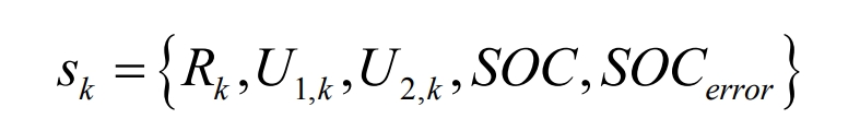
The selection of state variable types has a significant impact on control performance. Usually, it is necessary to observe and train fewer state variables to prevent the trained deep neural network from falling into local optimization. However, in the absence of key state variables, the Double DQN algorithm may not fully understand the interaction between the state transition process and the environment, resulting in difficulties in iteration and convergence. Therefore, the state variables selected in this article are shown in the equation.
(2) Action parameter settings
Need to discretize actions and set discretization steps reasonably. If the step size is too large or too small, it will affect the effectiveness of the algorithm. If the step size is too large, it will cause local optimization of the algorithm. If the step size is too small, it will increase the training time of the algorithm. According to the assumption, EKF provides the observation variance R in EKF for the Double DQN module, with the following action parameters:
(3) Reward function parameter settings
The reward function is used to evaluate the quality of action values under a given state, mainly relying on the estimation error of SOC, defined as:

The second part is the intelligent agent – Double DQN module, which utilizes the states s, actions a, and rewards r provided by EKF. It uses a greedy strategy to select actions to change the observation variance R in EKF. The generated experience samples (st, at, rt, s (t+1)) are stored in the experience playback pool, and then the randomly selected experience samples are played back every C steps to update the network parameters. The core of this section is to use greedy strategy to select actions to optimize the parameters of EKF. As the number of iterations increases, the output of the actions gradually stabilizes and the reward function obtains the optimal value.
3. Implementation process
Establish a simulation model using the reinforcement learning toolbox in Matlab and complete the simulation. The Matlab reinforcement learning toolbox can build a reinforcement learning environment that connects Matlab and Simulink. Among them, Matlab has built-in many instances of reinforcement learning, defining many Agent functions and related training parameter functions.
The Simulink simulation model based on EKF estimation of battery SOC established in the previous section is the foundation. Using the Matlab reinforcement learning toolbox, set corresponding observations, reward functions, end conditions, and Agent modules for training. The basic steps for implementing reinforcement learning are summarized as follows:
(1) Define the training environment;
(2) Set the critical target network and parameters in reinforcement learning;
(3) Set the training parameters for the reinforcement learning agent module;
(4) Set reinforcement learning training parameters;
(5) Debug and conduct simulation verification.
Next, we will expand on the above sections and provide some pseudo codes accordingly.
(1) Define training environment
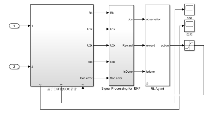
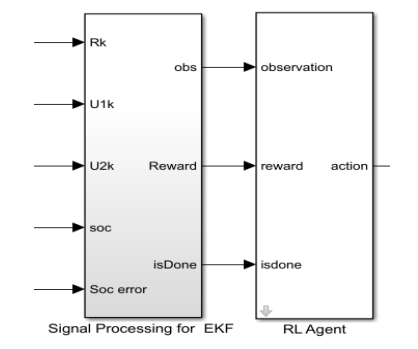
Defining a training environment refers to defining the environment in which an intelligent agent “Agent” runs, including the interface between the Agent and the environment and the dynamic model of the environment. This article further defines the interface between Agent and environment based on the Simulink model for battery SOC estimation based on EKF, which includes the definition of observation, action quantity, and reward function. The simulation model of Simulink for SOC estimation based on reinforcement learning optimization EKF is shown below.
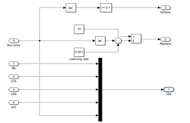
In this article, the signal format for measurement and action quantities is defined as a discrete variable (the signal format can be defined as either a discrete variable or a continuous variable). Insert a reinforcement learning Simulink module and define the observation, action volume, reward function, and end function. The reward function defined in it is described in the formula.
The inserted reinforcement learning Simulink module is shown in Figure 4.
The defined measurement, reward function, and end function are encapsulated in the “Signal Processing for EKF” module on the left. The five inputs on the left side of Figure 5 are Rk, U1, k, U2, k, SOC, and SOCorror, respectively. Output 1 on the right side is the observed measurement, output 2 on the right side is the reward function, and output 3 on the right side is the stop condition. The three values interact with the “RL Agent” module on the right, which outputs action actions. Define five actions in the action quantity in MATLAB to control the R value in the EKF based SOC estimation module using actions.
After defining the above variables and modules, create a reinforcement learning environment.
(2) Setting the network and parameters for the critical part of reinforcement learning
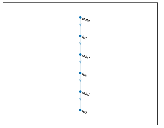
The dimensions of observation and action quantity defined in the previous step are used to establish a DNN network, which takes observation as input and selected actions as output, and establishes a 6-layer DNN network with 5 inputs and 5 outputs. The established DNN network is shown in Figure 6, which includes 1 input layer, 3 fully connected layers, and 2 activation layers.
Subsequently, critical parameters such as learning rate are set, and the established DNN network is trained for critical through the rlQValueRepresentation function. Training the critical module is very important because the basic Q-Learning of the double DQN algorithm implemented later is to estimate the feedback obtained and the reward to be obtained through critical.
(3) Set training parameters for reinforcement learning agent module
After establishing the above content, set up the agent in this step. The reinforcement learning toolbox contains various reinforcement learning agents, including Q-Learning, DQN, and DDPG. In this section, parameters for the DQN algorithm need to be set, including the sampling step size, double DQN algorithm, initial probability of greedy strategy, frequency of updating the target (critical network), cache experience buffer size, and the size of the small batch sample set MiniBatchSize extracted from the cache. The specific workflow is detailed in section 3.2.3. After setting the above parameters, use the rlDQNAgent function to define citic and the above parameters as Agents.
(4) Set reinforcement learning training parameters
After setting the agent parameters, the parameters for reinforcement learning training should also be defined. In this step, we will define the following parameters: maximum number of training cycles, maximum number of steps per training, stop training conditions, save agent conditions, etc.
Through the above definition, agents that meet the requirements can be saved during reinforcement learning training. After entering reinforcement learning training, the reinforcement learning episode manager will be opened, which can visually display the training process and training effectiveness, and the following indicators can be displayed:
EpisodeReward: The reward value obtained during this simulation process.
EpisodeSteps: The number of steps taken during this simulation process.
AverageReward: Calculate the average reward for the final certain number of simulation processes, set to 5 in the following figure, and this parameter can be specified through the trainOpts function.
TotalAgentSteps: Add the steps of all simulation processes.
EpisodeQ0: is the initial state value estimated by critical.
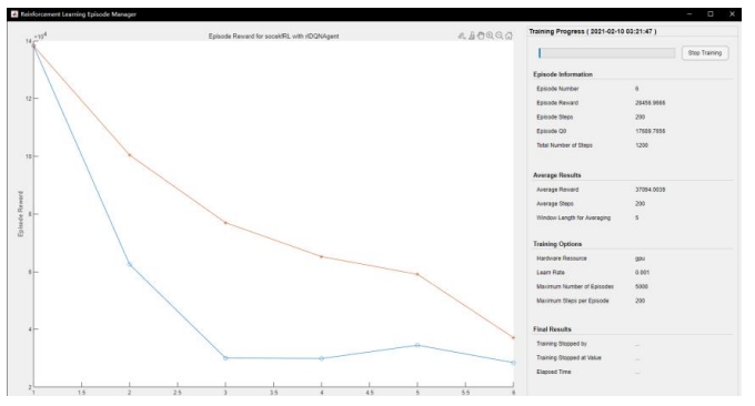
Through continuous learning and training of the algorithm, it should ultimately tend towards a stable state. AverageReward should tend towards EpisodeReward, and EpisodeReward should also gradually tend towards a stable state. If the Q function is the critical estimated state value, then episodeQ0 should gradually tend towards EpisodeReward.
(5) Debug and conduct simulation verification
The saved agent can be used to repeatedly verify the reinforcement learning effect, and the model can be optimized as much as possible through repeated debugging and verification. Generally speaking, the parameters that can be debugged come from the following aspects:
1) Training settings, including single simulation time, simulation step size, reset environment function, etc.
2) The configuration of the learning algorithm, namely the learning rate and other hyperparameters in the agent algorithm, can also be attempted to replace different agents.
3) Definition of reward signals
4) Action and observation signals
The partial Matlab pseudocode provided is as follows:
Open the established Simulink model
Define action quantity information, define action quantity as a discrete variable, including five actions
Define observable information as discrete variables, including five observables
Set the upper and lower limits of observation measurements
Define the established Simulink module as Agentblk
Using the rlSimulinkEnv function to comprehensively define the above signals as environments
Set the time and step size for a single simulation
Set the reset function env ResetFcn, restore the original state after each simulation
Set the DNN network with input as the observation dimension and output as the action quantity dimension, and set the hidden layers of DNN
Set up DNN network structure including input layer, fully connected layer, activation layer, and output layer
The most important parameter for setting the Critical parameter in this step is the learning rate α
Setting the DQNagent parameter in this section can affect the performance of Double DQN networks, discount factors, and greedy strategies
Initial probability, experience playback size n, maximum stored sample value N, small batch sample set size MiniBatchSize
Set the update frequency of the target (critical network)
Assign the set Agent parameters and Critical network to the Agent using the rlDQNAgent function
The most important parameters for setting reinforcement learning training parameters are the maximum training frequency, training stop value, and
Agent Save Values
If Training
Substitute the defined reinforcement learning agent, reinforcement learning environment env, and reinforcement learning training parameter trainingOpts to start training
Else
Import saved agents
End
Using Imported Agents to Realize Effect Reproduction
4. Simulation verification and analysis
| Hyperparameter | Parameter value |
| Step size | 7s |
| Learning rate | 0.001 |
| Discount factor γ | 0.99 |
| Initial Probability of Greedy Strategy | 0.6 |
| Experience playback size n | 100000 |
| Storage sample maximum value N | 100000 |
| MiniBatchSize | 64 |
| Target (critical network) update frequency | 4 |
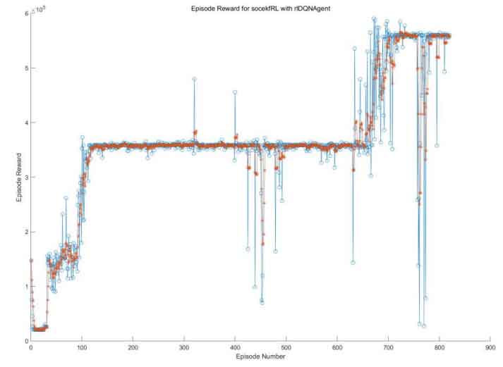
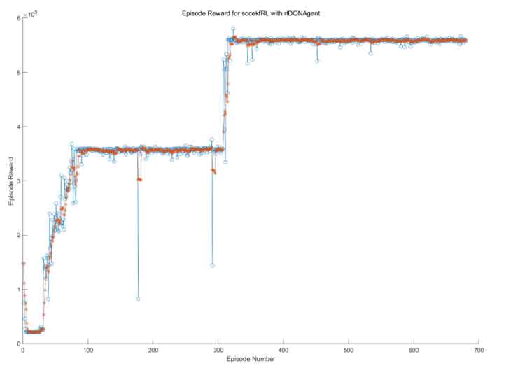
This article uses the Double DQN algorithm to improve the existing EKF based SOC estimation model. Due to time constraints, reinforcement learning training was conducted on the battery SOC during the 1000s time period, and compared with the DQN algorithm. Before starting the learning process of the algorithm, the hyperparameters in the algorithm should be set. Including discount factors γ、 The probability of storing the maximum value N of the sample and the greedy strategy ε The partial hyperparameters of the two algorithms, as well as the experience playback size n, are shown in Tables 1 and 2. Except for the Double DQN setting, all other hyperparameters are the same. The iterative rewards of the two algorithms are shown in Figure 8 and Figure 9, with the average reward shown in red.
| Hyperparameter | Parameter value |
| Step size | 7s |
| Learning rate | 0.001 |
| Discount factor γ | 0.99 |
| Initial Probability of Greedy Strategy | 0.6 |
| Experience playback size n | 100000 |
| Storage sample maximum value N | 100000 |
| MiniBatchSize | 64 |
| Target (critical network) update frequency | 4 |
Comparing Figure 8 and Figure 9, it can be found that the reward of the DQN algorithm is not stable and stays at the local optimal value for a long time. It is precisely due to the overestimation of the Q value that the DQN algorithm has poor stability and is difficult to quickly converge to the optimal effect. As the number of training increases, the reward value of the Double DQN algorithm stabilizes at a higher level, and the algorithm is relatively stable and converges faster. It has been proven that the Double DQN algorithm can solve the overestimation of Q values in the DQN algorithm and avoid the occurrence of dimensional disasters, which is also in line with the introduction of the Double DQN algorithm in the previous section.
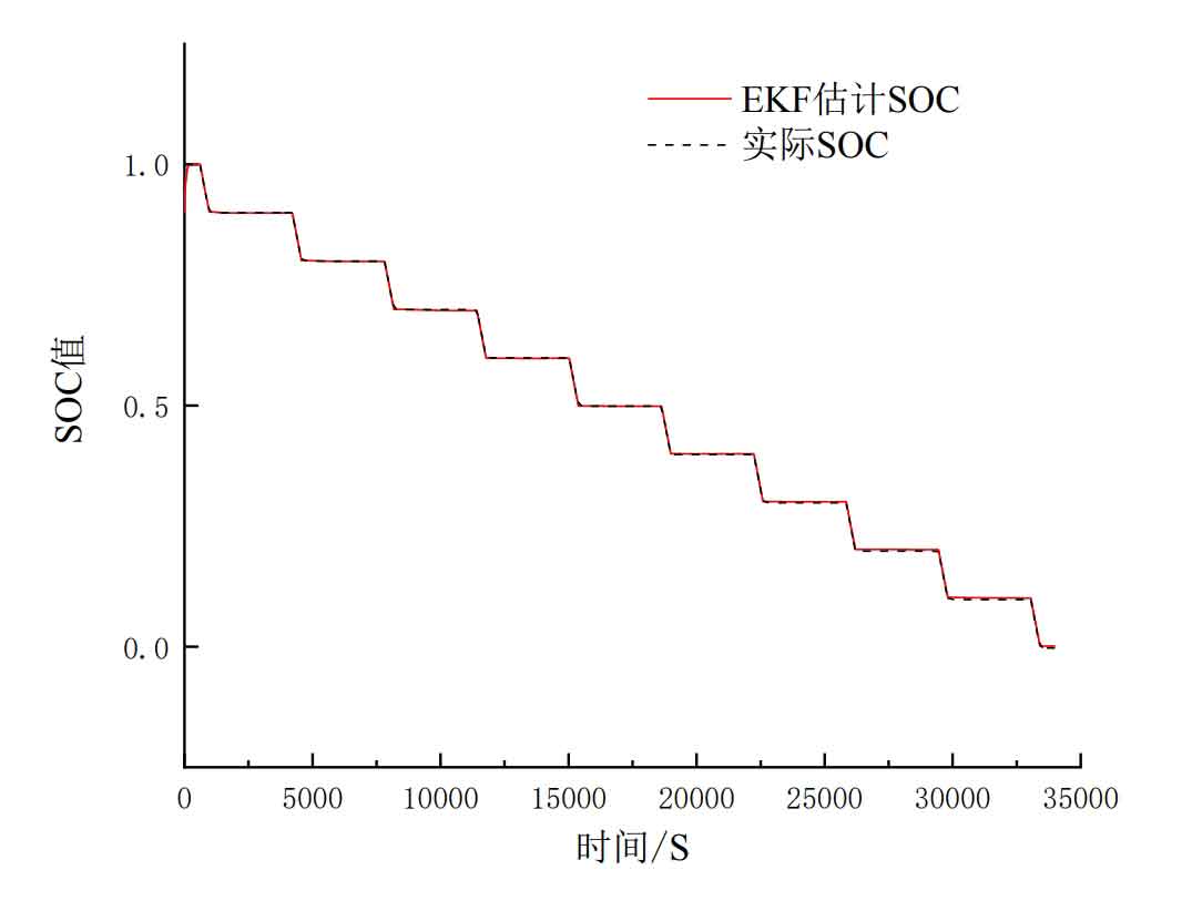
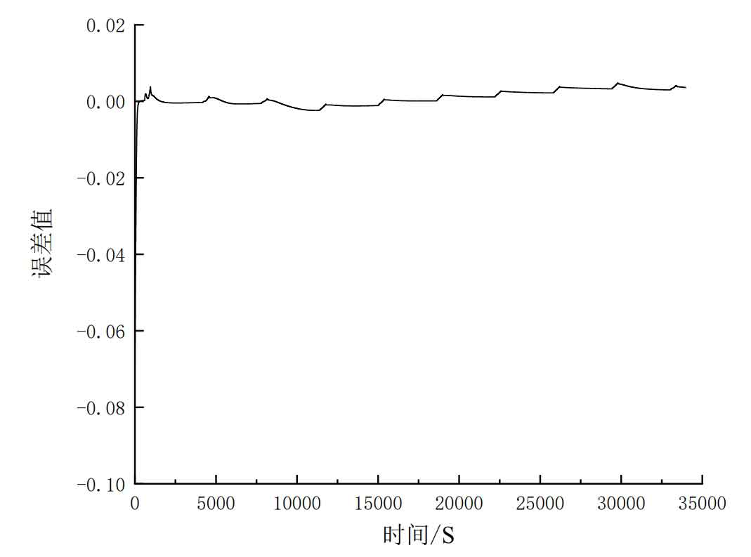
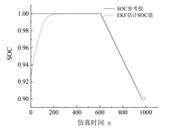
From Figure 10, it can be seen that the initial SOC value designed in this article is 0.9. When R=1, the comparison between the estimated SOC value by the EKF algorithm and the actual SOC value shows that the initial value of the estimated SOC by the EKF is set to 0.9, and the adjustment tends to the actual SOC, resulting in initial errors. In the later stage, the fluctuation errors are caused by the discharge and quiescence processes starting at 600s and 950s, respectively.
The following shows the performance of the simulated EKF algorithm for estimating SOC and the EKF algorithm optimized by reinforcement learning for estimating SOC. The simulation time of both models is set to 1000 seconds, and the parameters in the EKF algorithm are the same except for the changes in R values caused by actions taken in the double dqn algorithm. To avoid randomness, three sets of experiments were designed, with R values set to 1, 10, and 100 respectively, to observe the accuracy changes of the two models. And compare from two aspects to determine the effect of improved model accuracy. The first aspect is that by comparing the size of the MAE and MSE evaluation indicators of the three models in three sets of experiments, it can be concluded that the SOC estimation of the EKF optimized by Double DQN has an excellent evaluation indicator. The second aspect is that by comparing the adjustment response time of the early error and the later fluctuation error of the three models, it can be concluded that the SOC estimation of the EKF optimized by Double DQN shortens the adjustment response time of the early error and reduces the later fluctuation error. The error data and evaluation index statistical tables for three sets of experiments are presented below. Figure 11 shows the estimation errors of the three algorithms for SOC when the initial value of R is set to 100. We can conclude that the SOC errors estimated by the DQN algorithm and the Double DQN algorithm in Figure 11 converge to around 0 at 565s and 563s, respectively, while the SOC errors estimated by EKF did not converge to around 0 until the end of the simulation.
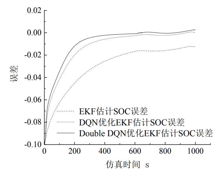
Figure 12 shows the estimation errors of the three algorithms for SOC when the initial value of R is set to 10. We can conclude that the estimation error of the EKF algorithm in Figure 12 converges to around 0 at 563s, while the estimation error of the SOC model optimized by the DQN and Double DQN algorithms converges to around 0 at 563s and 239s, respectively.
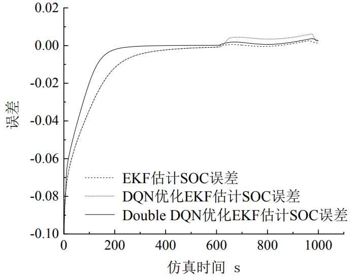
Figure 13 shows the estimation errors of the three algorithms for SOC when the initial value of R is set to 1. We can conclude that the EKF estimation of SOC and DQN in Figure 13, as well as the EKF estimation of SOC optimized by Double DQN, converge to around 0 at 195s, 149s, and 139s, respectively.
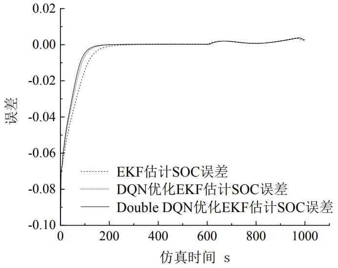
The evaluation indicators for the accuracy of the three types of SOC estimation models are shown in Table 3. Through analysis, it can be concluded that the optimized SOC estimation algorithm of the Double DQN algorithm has smaller errors than the other two algorithms. The evaluation indicators for the response time and error adjustment ability of the three SOC estimation models are shown in Table 4. It is not difficult to see that the optimized Double DQN algorithm has the fastest response time, but its later fluctuation error has no significant advantage.
| R-value | Model | MAE | MSE |
| R=100 | EKF estimated SOC | 0.0293 | 0.0013 |
| R=100 | DQN optimized EKF estimation of SOC | 0.0127 | 5.2088 × 10^-4 |
| R=100 | DoubleDQN optimized EKF estimation of SOC | 0.0093 | 3.9670 × 10^-4 |
| R=10 | EKF estimated SOC | 0.0091 | 3.6721 × 10^-4 |
| R=10 | DQN optimized EKF estimation of SOC | 0.0104 | 3.7331 × 10^-4 |
| R=10 | DoubleDQN optimized EKF estimation of SOC | 0.0060 | 2.4037 × 10^-4 |
| R=1 | EKF estimated SOC | 0.0052 | 1.9125 × 10^-4 |
| R=1 | DQN optimized EKF estimation of SOC | 0.0042 | 1.5138 × 10^-4 |
| R=1 | DoubleDQN optimized EKF estimation of SOC | 0.0040 | 1.4013 × 10^-4 |
In summary, the Double DQN optimized EKF estimation SOC algorithm proposed in this article has smaller error evaluation indicators and faster error adjustment response compared to the existing EKF algorithm and DQN optimized EKF algorithm, indicating that the optimized EKF model of the Double DQN algorithm is more accurate in estimating SOC.
| R-value | Model | Time to initially converge to 0 (s) | Maximum absolute value of fluctuation error generated after 600s |
| R=100 | EKF estimated SOC | Unconvergence | / |
| R=100 | DQN optimized EKF estimation of SOC | 900 | 0.002698254466185 |
| R=100 | Double DQN optimized EKF estimation of SOC | 565 | 0.002698254466185 |
| R=10 | EKF estimated SOC | 563 | 0.002702276188053 |
| R=10 | DQN optimized EKF estimation of SOC | 563 | 0.006212769938921 |
| R=10 | Double DQN optimized EKF estimation of SOC | 239 | 0.003744238821717 |
| R=1 | EKF estimated SOC | 195 | 0.003815589774170 |
| R=1 | DQN optimized EKF estimation of SOC | 149 | 0.003839334181852 |
| R=1 | Double DQN optimized EKF estimation of SOC | 139 | 0.003837448438975 |
5. Summary
This chapter mainly studies the estimation of the SOC value of lithium-ion batteries in energy storage systems using the EKF algorithm, and analyzes the impact of different parameter settings in the algorithm on the accuracy of the EKF algorithm. By using deep reinforcement learning to optimize the parameters of the extended Kalman filtering method and improving the original SOC estimation method, the estimation performance of SOC has been improved. This article introduces the process of optimizing the Double DQN of parameters in EKF for energy storage prediction. The state function of the equivalent circuit model and the function that causes errors in SOC estimation in EKF filtering are selected as the state variables, and the observation variance R in the control action EKF is changed to estimate the charged state SOC. Through simulation verification, it was found that the established reinforcement learning model can optimize the SOC estimation model based on the EKF algorithm, achieving faster adjustment and higher accuracy.