
1. Introduction
The integration of renewable energy sources, particularly solar photovoltaic (PV) systems, into power grids has accelerated globally. However, the intermittent nature of solar energy due to factors like irradiance fluctuations and temperature variations poses significant challenges to grid stability. Energy storage inverters, especially those combining PV systems with lithium battery storage, have emerged as critical solutions for mitigating these challenges. This study focuses on optimizing the control strategies for LCL-type photovoltaic energy storage inverters, addressing maximum power point tracking (MPPT), resonance damping, and harmonic suppression.
2. Photovoltaic Energy Storage System Modeling
2.1 Photovoltaic Cell Model
The output characteristics of PV cells are governed by the following equations:IL=Iph−Io[exp(AkTq(U+ILRs))−1]−RshU+ILRs
where Iph is the photocurrent, Io is the reverse saturation current, Rs and Rsh are series and shunt resistances, and A is the ideality factor. Under uniform irradiance, the power-voltage (P–U) curve exhibits a single peak, while partial shading introduces multiple peaks (Figure 1).
| Parameter | Value |
|---|---|
| Maximum Power (Pmax) | 266 W |
| Open-Circuit Voltage (Uoc) | 43.6 V |
| Short-Circuit Current (Isc) | 8.35 A |
2.2 Lithium Battery Storage System
The lithium battery pack is modeled as:Vb=Vo−RbIb−Q−∫IbdtK⋅Q+A⋅exp(−B∫Ibdt)
where Vb is the terminal voltage, Rb is internal resistance, and SOC (state of charge) is calculated as:SOC=100(1−Q∫Ibdt)
A bidirectional DC/DC converter regulates charging/discharging, maintaining a stable DC-link voltage (Udc=800 V).
2.3 Improved MPPT Algorithm
Traditional MPPT methods (e.g., Perturb and Observe, Incremental Conductance) struggle under partial shading. We propose a hybrid Cuckoo Search-Incremental Conductance (CS-INC) algorithm:
- Global Search Phase: CS algorithm rapidly locates the vicinity of the global maximum power point.
- Local Refinement Phase: INC algorithm fine-tunes the solution with adaptive step sizes.
Simulation Results:
- Uniform Irradiance: CS-INC achieves 98.57% accuracy in 0.14 s, outperforming CS (97.32% in 0.28 s).
- Partial Shading: CS-INC tracks the global peak (4591 W) in 0.19 s, while CS converges to a local peak (4330 W).
3. LCL Filter Design and Active Damping Control
3.1 LCL Filter Parameterization
The LCL filter attenuates high-frequency harmonics while minimizing power loss. Key design equations include:L1≥8ΔImaxfsUdc,C≤3⋅2πf0US25%Prated,fres=2π1L1L2CL1+L2
For a 10 kW system:
| Parameter | Value |
|---|---|
| L1 | 2 mH |
| L2 | 0.5 mH |
| C | 5 µF |
| fres | 3.56 kHz |
3.2 Inverter-Side Current Feedback Active Damping (ICFAD)
Passive damping introduces resistive losses. ICFAD emulates a virtual impedance Zeq(s):Zeq(s)=R⋅e−1.5sTs
This strategy suppresses resonance without physical resistors. The damping factor ζ is optimized as:ζ(ωr′)=2ωr′L1−KPWMKsin(1.5ωr′Ts)KPWMKcos(1.5ωr′Ts)
Bode Plot Analysis:
- Without Damping: Resonance peak at 3.56 kHz causes instability.
- With ICFAD: Resonance suppressed, phase margin > 45°, gain margin > 6 dB.
4. PI-Repetitive Composite Control Strategy
4.1 Repetitive Control with Odd-Harmonic Suppression
Traditional repetitive controllers suffer from slow dynamics. We propose a half-cycle internal model to target odd harmonics:GRC(z)=1−z−N/2Q(z)z−N/2Q(z)
where N=fs/f0 and Q(z) is a zero-phase low-pass filter.
4.2 Cascade PI-Repetitive Control
A cascade structure combines the dynamic response of PI with the harmonic suppression of repetitive control (Figure 2):GPI(s)=kp+ski,GRC(s)=1−e−sT0e−sTd
Digital Implementation:
- PI controller discretized using Tustin method.
- Repetitive controller implemented with a circular buffer for delay compensation.
4.3 Frequency-Adaptive Control
Grid frequency deviations degrade harmonic suppression. A fractional delay filter based on power series expansion adjusts the internal model period:H(z)=n=0∑Mn!(−1)n(Δ)ndzndnz−D
where Δ is the fractional delay and D is the integer delay.
Simulation Results:
- Steady-State: THD reduced from 4.8% (PI) to 1.2% (PI-Repetitive).
- Frequency Fluctuation (±2 Hz): THD remains below 1.5%.
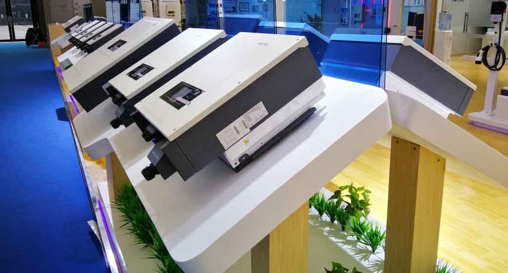
5. Hardware Implementation and Experimental Validation
A 10 kW prototype energy storage inverter was developed (Figure 3), with specifications:
| Component | Specification |
|---|---|
| DC Link Voltage | 800 V |
| Switching Frequency | 10 kHz |
| DSP Controller | TMS320F28335 |
| Grid Voltage | 220 V (rms), 50 Hz |
Key Results:
- Load Step Change (5 kW → 10 kW): Settling time < 20 ms, overshoot < 3%.
- THD Analysis: Grid current THD = 1.8% under nonlinear loads.
- Frequency Adaptive Test: THD < 2% for grid frequency variations (48–52 Hz).
6. Conclusion
This study presents a comprehensive approach to optimizing LCL photovoltaic energy storage inverters. The CS-INC algorithm enhances MPPT accuracy under partial shading, while ICFAD effectively suppresses LCL resonance. The proposed PI-repetitive cascade control reduces harmonic distortion, and frequency adaptation ensures robustness against grid fluctuations. Experimental results validate the strategies, achieving THD < 2% and dynamic response times < 20 ms. Future work will explore AI-based MPPT and multi-inverter synchronization for large-scale grid integration.
Formulas Summary:
- PV Output Current:
IL=Iph−Io[exp(AkTq(U+ILRs))−1]−RshU+ILRs
- LCL Resonance Frequency:
fres=2π1L1L2CL1+L2
- ICFAD Damping Factor:
ζ(ωr′)=2ωr′L1−KPWMKsin(1.5ωr′Ts)KPWMKcos(1.5ωr′Ts)
- Repetitive Control Transfer Function:
GRC(z)=1−z−N/2Q(z)z−N/2Q(z)
Tables Summary:
- Table 1: Photovoltaic cell parameters.
- Table 2: LCL filter design values.
- Table 3: Experimental prototype specifications.
This work advances the control methodologies for energy storage inverters, ensuring efficient and stable integration of renewable energy into modern power grids.