
1. Composition of photovoltaic microgrid system
The research on the microgrid structure and system is shown in Figure 1. The microgrid has a voltage level of 35kV and is composed of three sets of 1.5 MW photovoltaic power generation units, a set of 2 MW (2MW · 2h) battery energy storage system, and several loads.
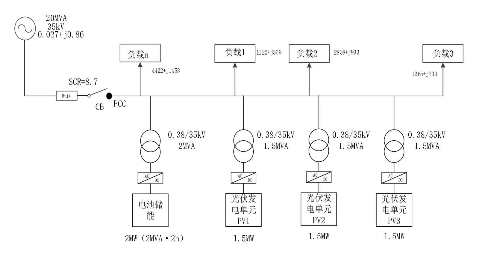
PCC is the point of common coupling (PCC) of the system, and by controlling the circuit breaker CB, the microgrid can operate in both grid connected and island mode. The short circuit capacity of the PCC system is 56.7MVA, and the rated DC power of the microgrid system is 6.5MW, consisting of:
In the formula, Kscr is the short-circuit ratio of the system, Sac is the short-circuit capacity of the AC bus, and PdN is the rated DC power. The short circuit ratio of PCC is 8.7. Therefore, the main grid is very powerful and stable for photovoltaic power generation systems and battery energy storage systems in microgrids. The penetration rate of photovoltaic power generation in microgrid systems is calculated by the following equation:
In the formula: Ppv max is the maximum power ratio of the photovoltaic power generation system, Pd max is the maximum load of the microgrid (all under standard conditions, radiation intensity=1000W/m) ², Battery temperature=25 ℃), assuming that the maximum load of the microgrid is approximately equal to the maximum capacity of the main grid of 20MVA. The penetration rate of photovoltaic power generation in this system, P%, is 22.5.
2. Modeling and analysis of photovoltaic power generation systems
2.1 Structure of photovoltaic power generation units
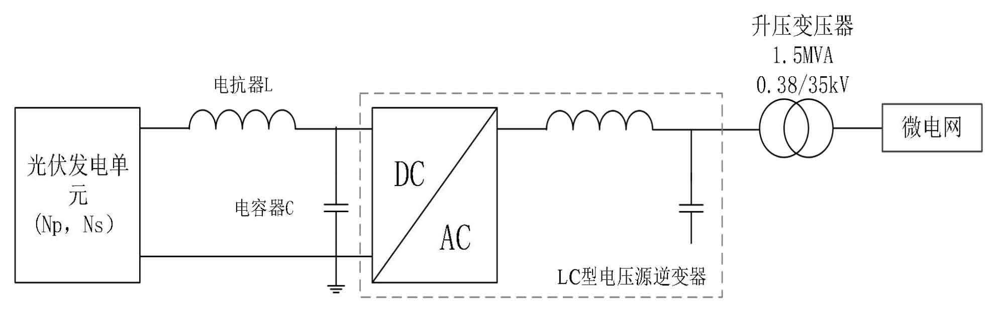
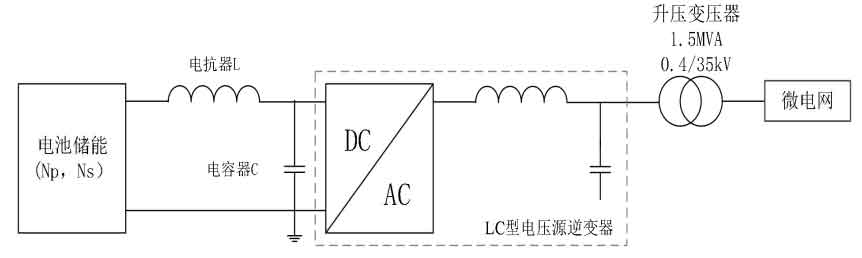
Figure 2 is the structural diagram of the photovoltaic power generation system studied in this article, which includes a photovoltaic power supply, DC reactor, DC capacitor, LC type voltage source inverter, and finally connected to the microgrid through a step-up transformer. The microgrid has three power generation units, each with a rated power of 1.5MW. An ideal DC inductor is connected in series at the output end of the photovoltaic power supply for harmonic suppression, with a value of 5 µ H. The rated capacity of the step-up transformer is 1.5MVA, and the transformer connection group is Dyn11. The voltage level is 0.38/35kV. In this article, the focus will be on discussing and analyzing the models of photovoltaic power sources and LC type voltage source inverters.
2.2 Characteristics and models of photovoltaic cells
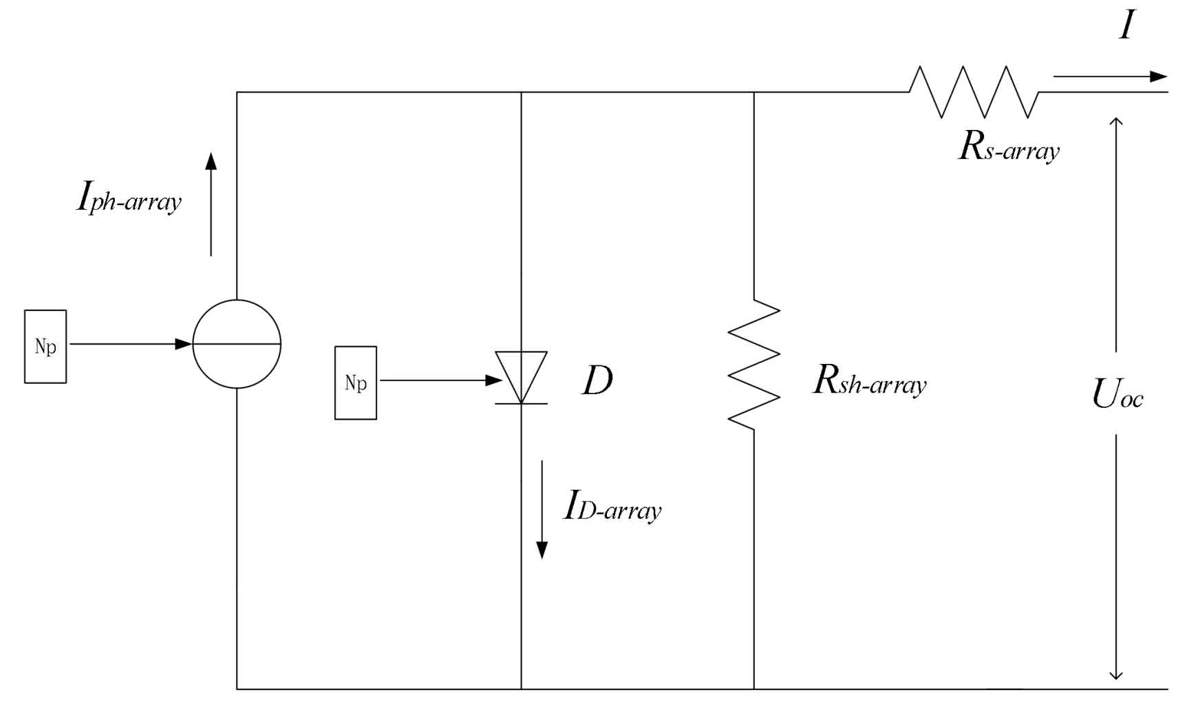
A photovoltaic array usually consists of many photovoltaic cells in series and parallel, and the equivalent circuit of a single photovoltaic cell is shown in Figure 3.
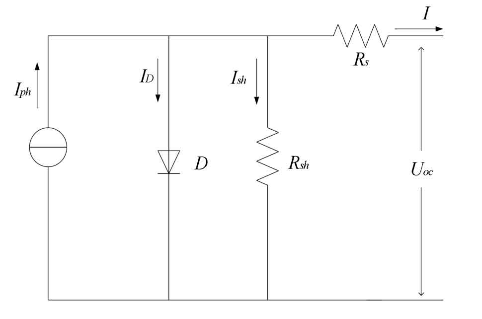
Among them, pH I is the photogenerated current; Uoc is the voltage of the photovoltaic cell; DI is the current passing through the PN junction. Rs is the series resistance; Rsh is a parallel resistor.
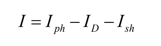
According to Kirchhoff’s current law, the output characteristic formula of photovoltaic cells is listed in Figure 3:
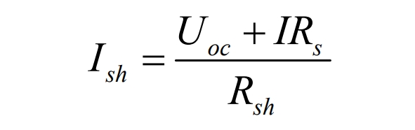
The current Ish flowing through the parallel resistor Rsh can be expressed as:
The current and voltage relationship of the PN junction satisfies the following equation:
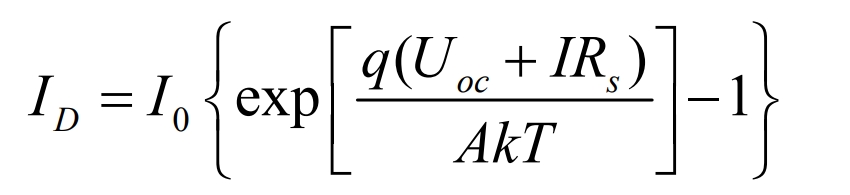
I is the reverse saturation current of the diode; Q is the amount of electronic charge, with a value of 1.6 x10 ^ -19 C; A is the ideal factor of PN junction; Generally taken as 1; T is the ambient temperature; K is the Boltzmann constant with a value of 1.38 x 10 ^ -23 J/K.
By combining the formulas, it can be concluded that:
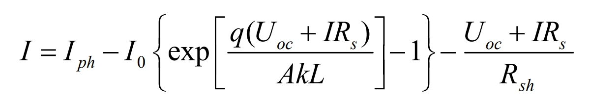
In the formula, Rsh>>U+IRs, making U+IRs/Rsh very small and negligible relative to the photo generated current source Iph. And because Rs are very small, IL Rs are<<Uoc.
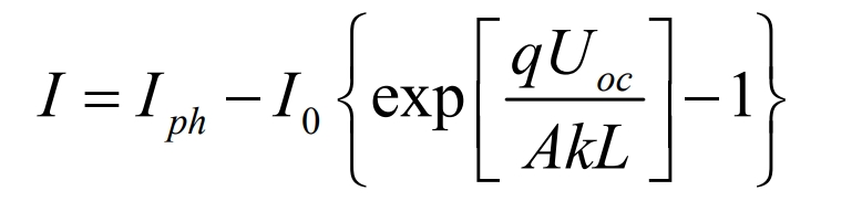
Based on the above conditions, the formula can be simplified as follows:
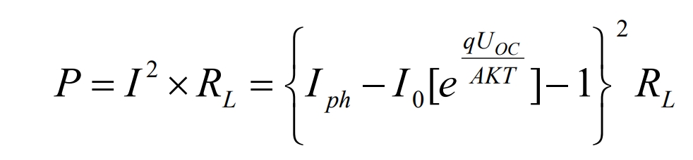
If the external load of the photovoltaic cell is RL:
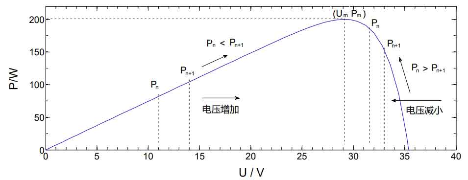
Establish a photovoltaic array simulation model on the Matlab/Simulink platform to obtain P-U curves at constant temperature, variable light intensity, and constant light intensity, as shown in Figures 4 and 5. The main parameters are Voc=35.7V, Vm=28.8V, Isc=7.44A, Im=6.94A, a=0.0025, b=0.5.
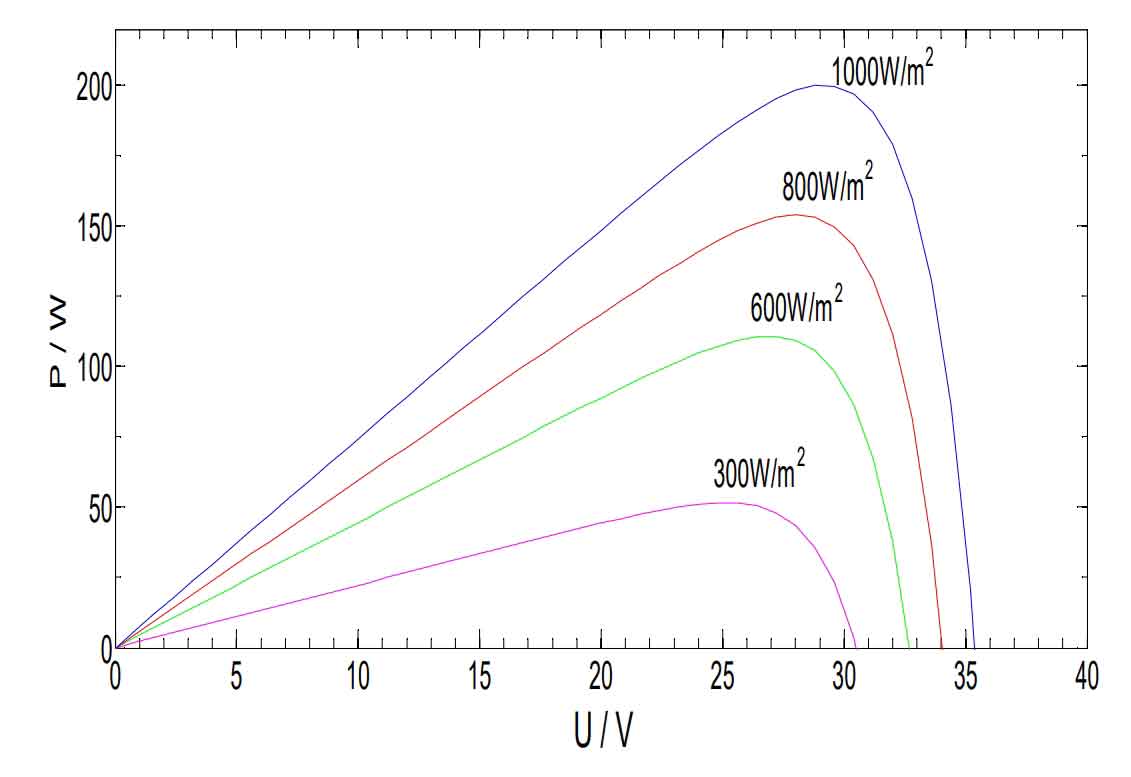
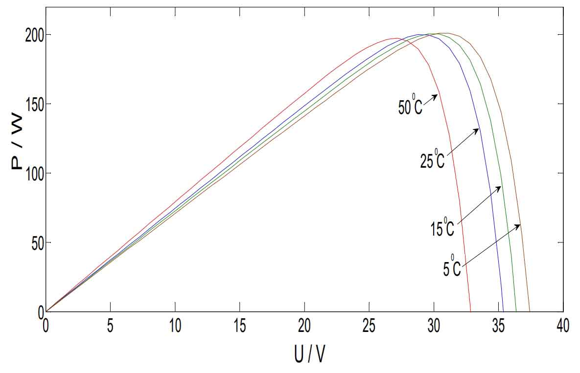
Through observation, it can be seen that the P-U characteristic curves in Figures 4 and 5 exhibit nonlinear changes, increasing first and then decreasing, reaching a maximum point during this process. When the maximum power and voltage at the maximum power point increase with the increase of light intensity, they decrease with the increase of temperature.
Due to the fact that photovoltaic power generation systems are composed of photovoltaic cells in series and parallel, the number of them needs to be considered during the modeling process, where Np and Ns are the total number of photovoltaic cells in parallel and series, respectively
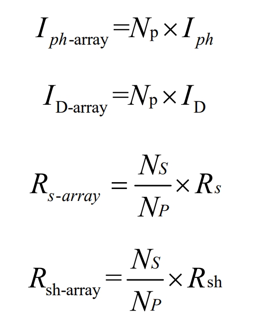
Modeling the photovoltaic array in the Matlab software platform is shown in Figure 6. Based on the number of series and parallel batteries in the photovoltaic array and the formula, D-array I and sh array I can be used to represent the output of the photovoltaic power supply, as shown in Figures 4 and 6. The rated power of each photovoltaic power generation unit in the microgrid is 1.5 MW. In this article, 270-60P polycrystalline photovoltaic modules are selected as photovoltaic cells, with 280 sets in parallel and 20 sets in series. In the above equation, Np=280 and Ns=20. Table 2-1 provides the parameters of photovoltaic modules under standard conditions (irradiation intensity S=1000 W/m2 and temperature T=25 ° C).
| Model | 270-60P | Maximum power | 270W |
| Working current | 8.73 A | Short circuit current | 9.18 A |
| Working voltage | 30.9 V | Open circuit voltage | 38.4 V |
2.3 Mathematical model of three-phase bridge voltage source inverter with LC filter
Figure 7 shows the topology of the three-phase bridge voltage source inverter system with LC filter studied in this paper, with a rated voltage of 0.6 kV DC/0.38 kV AC. The rated value of the DC side capacitor C1 is 280 mF, and the AC side is connected to an LC type grid connected filter represented by LC in the figure, where L=37 µ H and the filtering capacitor C=5.1 mF. The direct current generated by the photovoltaic power supply is converted into alternating current here, which is filtered and processed with sinusoidal pulse width modulation (SPWM) to obtain the required sinusoidal alternating current. It is connected to the low-voltage side of a rated 1.5 MVA transformer with a transformation ratio of 0.38/35kV.
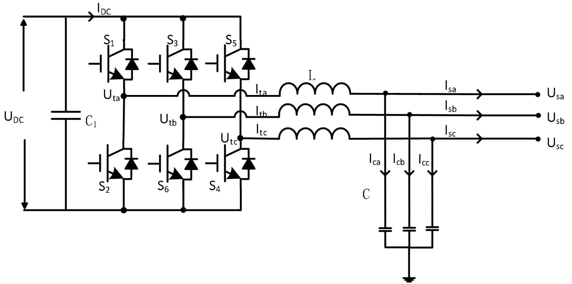
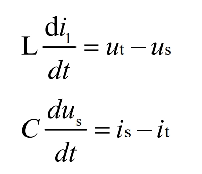
In the figure, ut represents the output terminal voltage of the inverter, and us represents the output terminal voltage. I1 and i2 are the currents on the filter inductance and filter capacitor, respectively, while i3 is the current flowing through the low-voltage side of the transformer. According to Kirchhoff’s law of voltage and current, the voltage on the inductor and the current on the capacitor are:
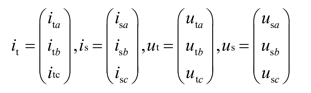
Where u and i are all three-phase AC vectors:
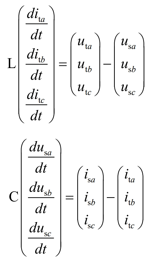
Bringing the formula into can lead to:
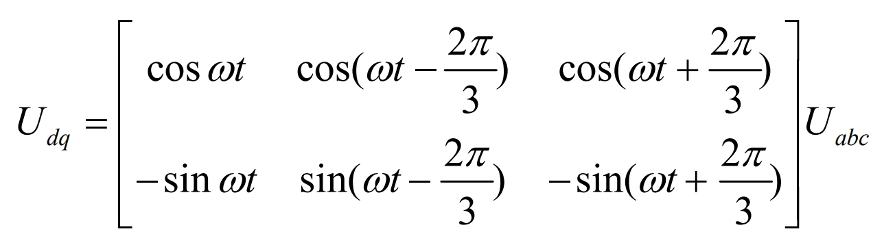
The above is a mathematical model of a three-phase inverter in a stationary coordinate system, which has the advantages of being intuitive and easy to understand. However, the various AC signals in the mathematical model are time-varying and complex to control. Therefore, the mathematical model in a three-phase stationary coordinate system is generally converted into a two-phase (d, q) rotating coordinate system for control, also known as dq transformation. The dq transformation formula is:
After dq transformation, we can obtain:
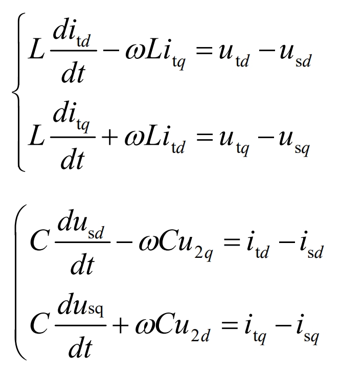
The formula is the mathematical model of a three-phase inverter in the dq coordinate system.
3. Modeling and Analysis of Battery Energy Storage System
3.1 Structure of battery energy storage system
Figure 8 shows the structure diagram of the network battery energy storage system studied in this article, which is similar to Figure 2-2. The photovoltaic power supply is replaced by lithium batteries at the power supply end. The rated voltage of the inverter is 0.7 kV DC/0.38 kV AC, the value of the DC side reactor is 20 µ H, the rated value of the DC side capacitor C is 40mF, the AC side LC filter L=37 µ H, C=5.1 mF, the rated capacity of the step-up transformer is 2MVA, and the voltage to voltage ratio is 0.38/35kV.
3.2 Mathematical Model of Battery Energy Storage System
Lithium ion batteries are an electrochemical device that stores electrical energy in an electrochemical form and can provide direct current output. At the same time, lithium-ion batteries have the characteristics of high working voltage, small size, light weight, no pollution, small self discharge, and long cycle life. Therefore, this article selects lithium-ion batteries as energy storage systems. According to the internal parameters of the battery, a battery array is formed through series parallel combination to provide the required rated voltage and current value. In this article, the working voltage of each lithium-ion battery is 3.5V and the working current is 120Ah. Build a battery pack module by connecting 24 batteries in parallel, and then connect 400 battery modules in parallel and series. There is the following formula:
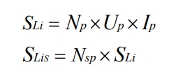
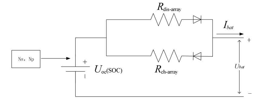
In the formula: SLi is the capacity of a single battery pack module, Up and Ip are the rated voltage and current of a single battery, Np is the number of parallel batteries, Nsp is the number of series parallel battery modules, and the calculated capacity of the battery energy storage system is 4MVA · h. The maximum output power of the energy storage system is 2MW. For the equivalent circuit model of a battery, its physical meaning is clear and can be analyzed using mathematical formulas, making it more convenient to identify the parameters of the battery model. As shown in Figures 9, the voltage source resistor equivalent model of the battery [49]. This model avoids the complex calculation of the electrochemical process inside the battery and is suitable for studying the state of the battery during charging/discharging processes in the short or long term.
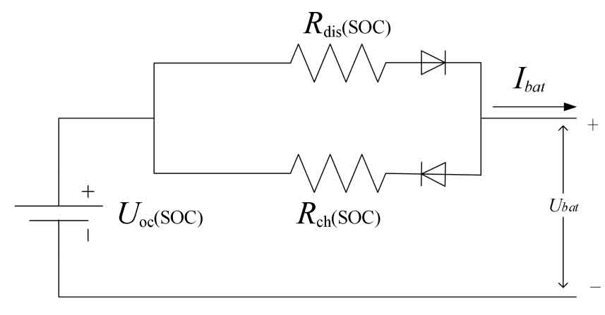
The battery model consists of a DC voltage source and two series resistors Rch and Rdis. Uoc is the open circuit voltage of the battery, and the series resistors Rch and Rdis represent the power loss during charging and discharging operations. It can be seen that Uoc, Rch, and Rdis are functions of the battery SOC and its operating temperature (T), where the State of Charge (SOC) of the battery is defined as the ratio of the remaining battery capacity to its rated capacity, with the following relationship:
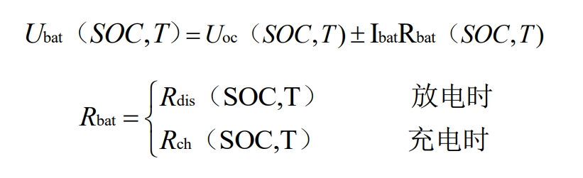
Without considering the changes in battery temperature, Uoc, Rch, and Rdis are only functions of SOC. For SOC, in order to prevent excessive battery charging and discharging, its value should be within a normal range, and SOC can be expressed as:
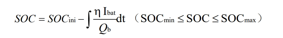
Among them, SOCini represents the initial charging state of the battery, Qb is the capacity (kAh) of the battery, where SOCini represents the initial charging state of the battery, Qb is the capacity (kAh) of the battery, and Δ bat is the output current (A) of the battery. When the battery is charged and discharged, it is represented as either negative or positive. is defined as the efficiency of the battery. Determined by the following equation:
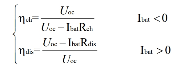
Among them η Ch is the charging efficiency, and dis is the discharge efficiency. From the above equation, it can be seen that the rate of charging and discharging of the battery (i.e| η The size of bat | determines the efficiency of the battery, and a higher charging and discharging rate will reduce the efficiency of the battery. In current research on battery pack SOC, series-parallel battery packs are usually intuitively regarded as a large battery, modeled to estimate the state of charge. Therefore, the number of battery modules is considered in the modeling process, where NP and NS are the number of battery modules connected in parallel and series, respectively
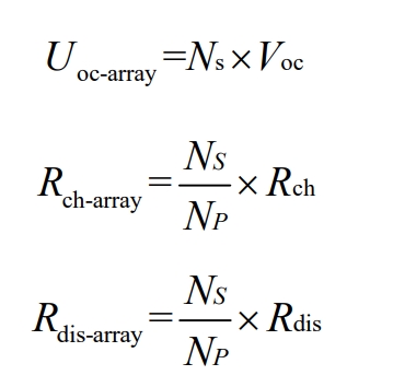
Modeling the battery energy storage system on the Matlab software platform is shown in Figure 10. The rated power of the battery pack is 2MW (2MW · 2h), which means that the energy storage system can provide a maximum power output of 2MW for up to 2 hours. During the modeling process, the input of the voltage source is controlled by adjusting NP and NS, as well as Rch and Rdis. Among them, NP=42 and NS=1. The layout structure and parameters of energy storage batteries are shown in Table 2.
| Single battery capacity | 120Ah (2.60Ah) 3.5V |
| Single battery module | 24 single batteries in series |
| 100kW | 10 battery modules in series |
| 2MW (2MW · 2h) | 42 100kW battery modules in parallel connection |
| Minimum voltage | 672 V |
| Maximum voltage | 84 |
4. Analysis and Improvement of Maximum Power Point Tracking (MPPT) Method
By analyzing the characteristics and models of photovoltaic cells, in order to improve the efficiency of photovoltaic power generation units to a certain extent, the maximum power point tracking (MPPT) method is more commonly used, such as disturbance observation method, constant voltage method, and conductivity increment method. This section mainly analyzes disturbance observation methods and proposes an adaptive variable step size disturbance observation method based on this, which enables the disturbance step size to achieve self adjustment. Then, by controlling the duty cycle of the Boost boost circuit, the maximum power tracking of the photovoltaic system is achieved.
4.1 Principles of disturbance observation method
The disturbance observation method is simple and highly feasible. It can change the voltage and current values of the photovoltaic system through disturbance, and then combine the calculation method of P=UI to obtain the output power. Compare the two power values measured before and after, and if it is found that the latter is greater than the former, output the same disturbance direction. If the latter is smaller than the former, it outputs the opposite interference direction. Pk and Pk-1 in the figure represent the current and previous sample values, respectively. The schematic diagram of the perturbation observation method is shown in Figure 11. Its drawbacks are:
(1) The system cannot balance tracking accuracy and response speed: if the step size is too large, power fluctuations may occur, resulting in insufficient tracking accuracy; If the step size is too small, the tracking time will increase, and the system may also work at low power output points for a long time.
(2) The final result of the system is continuous oscillation in a small range near the maximum power point.
(3) When the external environment constantly changes, the disturbance observation method may experience significant power fluctuations and may even cause misjudgment.
4.2 MPPT principle based on adaptive variable step size disturbance observation method
Through analysis, it can be concluded that the disturbance observation method cannot simultaneously track accuracy and response speed. If the power changes before and after the comparison of the two powers are not significant, it indicates that the output power of the power supply is close to the maximum power point, and there should be a small change in step size.
When the power changes significantly in the last two times, it indicates that the distance between the output power of the photovoltaic power source and the maximum power point is still relatively far, and the change step should be larger. This approach can reduce power fluctuations and also accelerate tracking speed.
Reasonably set the step size so that the steps d (k), d (k+1) before and after meet the following requirements:
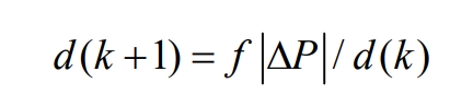
In the formula, d (k) is the step size of the disturbance voltage, which varies between 0 and 1; Δ P=P (k) – P (k-1), where
Changes in power; F is a constant, reflecting the sensitivity of adaptive adjustment.
When the power changes Δ P is very small, i.e| Δ P | Very small| Δ P |/d (k) is also very small, d (k+1) is very small, that is, the step size becomes smaller; When there is a significant change in power, i.e| Δ P | Very large| Δ P |/d (k) is also large, and d (k+1) is large, which means the step size becomes larger, which improves the speed of tracking maximum power. In order to reduce the complexity of the improved disturbance method in design, the photovoltaic power generation system is connected to the boost circuit, and the impedance is matched by adjusting the duty cycle D of the PMW signal in the boost circuit to achieve maximum power tracking.
4.3 Model based on adaptive step size perturbation observation method MPPT
The basic principle of perturbation observation method is to continuously search and find during tracking Δ The point at P=0, but in reality, finding this point is very difficult. Continuous disturbance causes a certain degree of power oscillation, resulting in energy loss in the system and thus affecting the accuracy of tracking. In order to reduce the oscillation of the system, the parameter e is introduced to Δ Discriminate at time P, when| Δ When P |<e, we assume that it is already operating at the maximum power point, and at this point, the disturbance should be stopped. The flowchart of the improved adaptive variable step size disturbance observation method is shown in Figure 12.
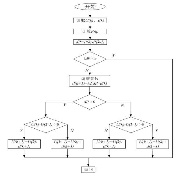
This method is basically consistent with the principle of traditional disturbance observation method, and it also seeks the maximum power point through continuous disturbance. However, the difference is that the step size of disturbance will change with the change of the working point, thereby improving the response speed of the system and improving its work efficiency. The MPPT control algorithm is implemented by establishing an M file of the S function, and is combined with the Matlab/Simulink simulation platform. The input signal of the S-function is the current output power of the photovoltaic power source; The duty cycle D is the output signal, which is the result calculated by the MPPT control algorithm.
4.4 Simulation analysis of photovoltaic cell MPPT
This article compares the adaptive variable step size disturbance observation method with the variable step size disturbance observation method proposed in reference on the Matlab/Simulink platform. The circuit simulation model for photovoltaic array implementation of MPPT is shown in Figure 2-13. The parameters are shown in Table 2. The parameters of the Boost circuit are: L=10×10 ^ -3H, C=300 x 10 ^ -6 F, C1=100X10 ^ -5F, R=300 Ω.
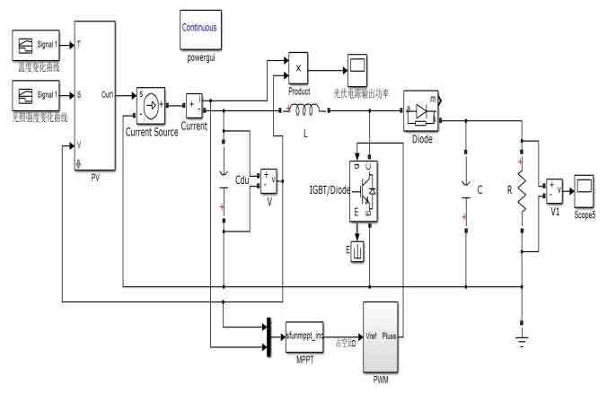
| Maximum power under standard conditions | 140W |
| Peak operating current | 7.94A |
| Peak operating voltage | 17.7V |
| Short circuit current | 8.58A |
| Open circuit voltage | 22V |
| Current temperature coefficient a | 0.0025/0C |
| Light intensity coefficient b | 0.5 |
| Voltage temperature coefficient c | 0.00288/0C |
Figure 14 shows the changes in temperature and light intensity, while Figure 15 shows the output power curve obtained by the variable step perturbation observation method. Figure 16 shows the simulation results of photovoltaic cell output power obtained by the improved adaptive variable step disturbance method.
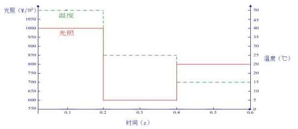
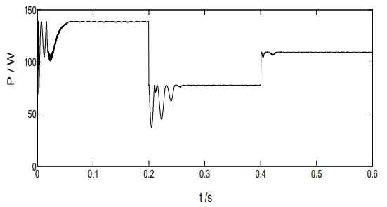
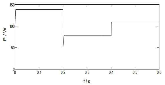
The changes in temperature and light intensity are shown in Figure 14. It can be seen that at 0.2s, the external temperature and light intensity both changed, with the external temperature dropping from 50 ℃ to 25 ℃ and the light intensity increasing from 1000W/m ² Reduce to 600W/m ², At 0.4 seconds, the external temperature continued to decrease to 15 ℃, while the light intensity increased to 800W/m ²。 Figure 15 shows the power output of the photovoltaic power supply using the variable step perturbation method when temperature and light intensity change. According to the figure, it can be seen that reaching the maximum power of the photovoltaic array takes a long time and there are certain fluctuations in power, especially when the external conditions change by 0.2s and 0.4s, the output power changes greatly. Therefore, it can be seen that if the external environment changes, it will bring about more energy loss, This results in a decrease in tracking accuracy. Figure 16 shows the waveform of the output power of the photovoltaic power supply obtained by introducing the improved step size adaptive disturbance method when the temperature and light intensity change. It can be intuitively seen that the time required for the output power to reach 140W and maintain stability in the graph is very short and almost negligible. Moreover, at the time of changes in external conditions of 0.2s and 0.4s, there is no significant change in the final output power, This characteristic makes the improved step size adaptive perturbation method more prominent in environments with frequent and rapid changes in temperature and lighting.
5. Summary
Introduced the composition of the photovoltaic microgrid studied in this article, and established mathematical models of photovoltaic power generation units and battery energy storage systems. In the photovoltaic power generation process, the focus was on discussing and analyzing the mathematical model and characteristics of photovoltaic cells, as well as the system structure of voltage source inverters (DC/AC). Then, the components of the battery energy storage system were introduced, and a voltage source resistor equivalent circuit model was established. Its working characteristics were analyzed, and the mathematical model of battery energy storage used was constructed. On the basis of the traditional variable step size disturbance observation method, an adaptive variable step size disturbance observation method is proposed to achieve automatic adjustment of disturbance step size. Simulation comparison shows that when external conditions change, the improved step size adaptive disturbance method can improve the tracking speed of the maximum power point and reduce the amplitude of power fluctuation, greatly improving the efficiency and utilization of photovoltaic power generation.