
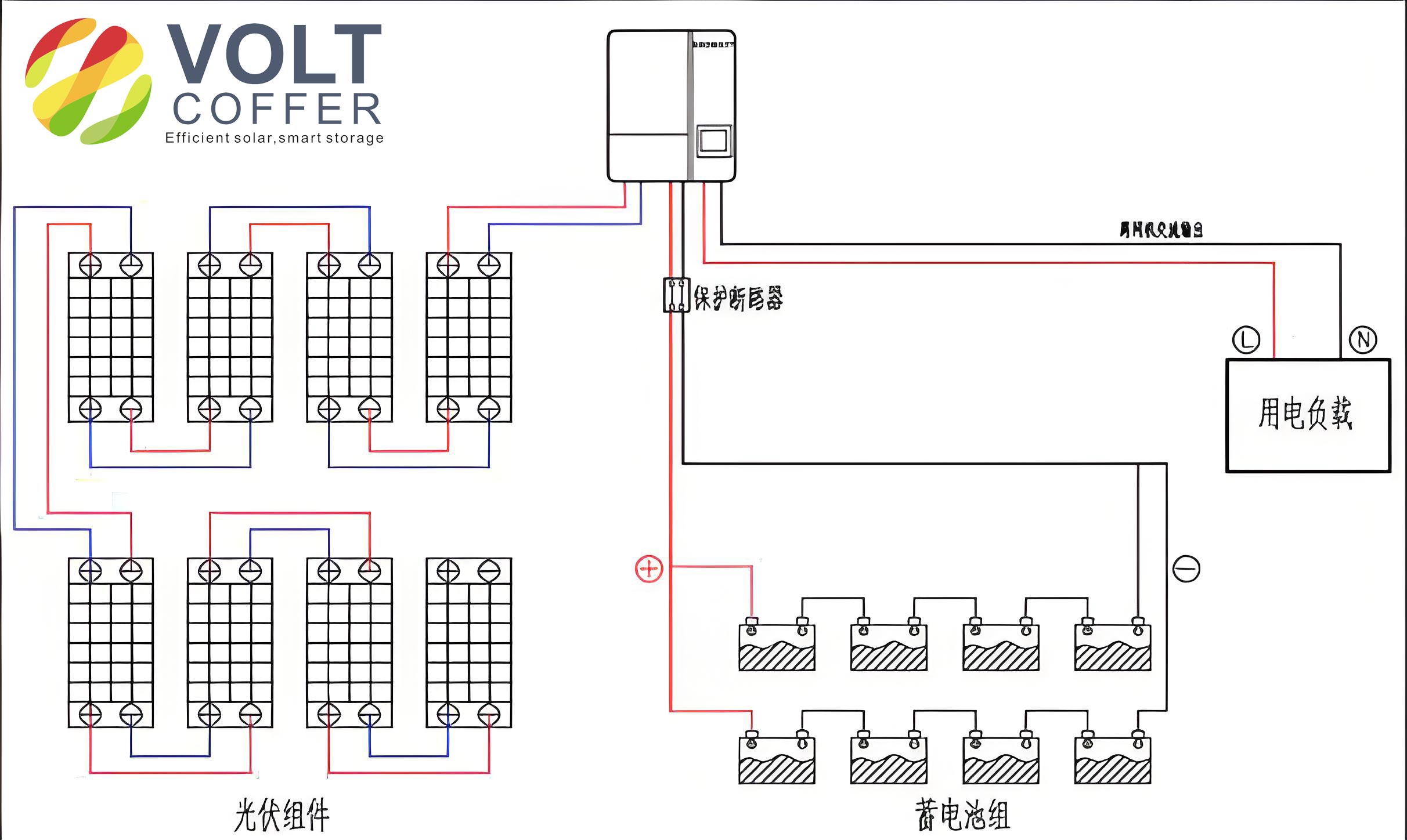
As the global energy crisis and environmental pollution intensify, the adoption of renewable energy sources, particularly wind and solar power, has become a critical focus worldwide. Off-grid solar systems offer a viable solution for providing clean and reliable electricity to remote areas and islands, where grid connectivity is challenging. These systems typically consist of photovoltaic (PV) panels for power generation, battery storage for energy retention, transmission components like cables and inverters, control systems including controllers and protective devices, and load systems comprising AC and DC loads. This article presents a comprehensive optimization design methodology for off-grid solar systems, focusing on maximizing power supply reliability and minimizing lifecycle costs. By developing mathematical models for PV generation, battery storage, system efficiency, and load management, we aim to enhance the performance and economic viability of these systems. The approach includes calculating optimal PV panel orientation, tilt angles, and spacing, as well as determining the ideal configuration of PV capacity and battery storage through iterative analysis. A case study demonstrates the practical application of this methodology, ensuring that the system meets load demands efficiently. Throughout this discussion, the term ‘off grid solar system’ will be emphasized to highlight its relevance in sustainable energy solutions.
The foundation of designing an efficient off-grid solar system lies in accurate mathematical modeling of its components. The power output of PV panels depends on the solar radiation incident on their surface, which is influenced by factors such as radiation intensity and the panel’s orientation. To maximize solar energy capture, it is essential to optimize the azimuth and tilt angles of the PV panels. For a fixed tilt angle without shading, the optimal azimuth angle, denoted as \( Z_c \), is derived by considering the direct radiation component. Since scattered radiation is relatively independent of orientation, the focus is on direct radiation. By differentiating the direct radiation intensity with respect to the azimuth angle, we find that the optimal value is \( Z_c = 0 \), meaning the panels should face true south in the Northern Hemisphere for maximum exposure.
Similarly, the optimal tilt angle \( \beta \) is determined to maximize annual energy yield, accounting for both direct and diffuse solar radiation. This involves solving for the tilt that maximizes the total radiation incident on the panel surface. The total radiation on a tilted surface includes direct, diffuse, and reflected components, and it can be modeled using the Hay anisotropic sky model for diffuse radiation. The instantaneous power output of the PV system at time \( t \) is given by:
$$w_{pv}(t) = \frac{H_T(t)}{1000 H_0} P_{0pv} F_t(t) F_s F_\mu F_0$$
where \( H_T(t) \) is the solar radiation on the tilted surface (in W/m²), \( H_0 \) is the reference radiation (typically 1000 W/m²), \( P_{0pv} \) is the rated power of the PV panel, \( F_t(t) \) is the temperature correction factor, \( F_s \) is the soiling factor accounting for dust accumulation, \( F_\mu \) is the performance mismatch factor, and \( F_0 \) represents other factors causing power degradation. This equation allows for precise estimation of energy generation under varying conditions, which is crucial for sizing the off grid solar system appropriately.
Battery storage is a critical component in off-grid solar systems, ensuring energy availability during periods of low solar insolation. The battery’s state of charge (SOC) varies based on the balance between PV generation and load demand. The battery can be in charging, discharging, or idle states, depending on whether the PV output exceeds, falls short of, or equals the load requirement. Let \( P_{rea}(t) \) represent the actual PV power available at time \( t \), and \( P_{ref}(t) \) denote the load power requirement. The battery’s capacity \( E(t) \) at time \( t \) is updated as follows:
When \( P_{rea}(t) > P_{ref}(t) \), the battery charges:
$$E(t) = E(t-1) + P_c(t) w_c \Delta t$$
where \( P_c(t) \) is the charging power, \( w_c \) is the charging efficiency (typically between 0.6 and 0.8), and \( \Delta t \) is the time interval.
When \( P_{rea}(t) \leq P_{ref}(t) \), the battery discharges:
$$E(t) = E(t-1) – \frac{P_d(t) \Delta t}{w_d}$$
where \( P_d(t) \) is the discharging power and \( w_d \) is the discharging efficiency (also between 0.6 and 0.8).
In idle states, such as when PV generation matches load demand or the battery is at minimum or maximum SOC, the capacity remains unchanged: \( E(t) = E(t-1) \) and \( P_b(t) = 0 \). These dynamics ensure that the off grid solar system maintains a reliable energy supply, even under fluctuating weather conditions.
To evaluate the overall performance of an off-grid solar system, it is essential to calculate the system efficiency, which encompasses losses at various stages. The key efficiency components include PV array efficiency, combiner box efficiency, DC line losses, inverter efficiency, controller efficiency, and AC line losses. The system’s overall efficiency determines the net energy available to the load. The PV array efficiency \( \eta_{Amean} \) over a period \( \tau \) is defined as:
$$\eta_{Amean} = \frac{w_{PV}}{A \times H_T}$$
where \( w_{PV} \) is the energy output from the PV array, \( A \) is the effective area of the array, and \( H_T \) is the total radiation on the tilted surface. Factors like internal resistance, shading, and material defects can reduce this efficiency.
The combiner box efficiency accounts for losses due to diodes, with the efficiency \( \eta_2 \) given by:
$$\eta_2 = 1 – \xi_2$$
$$\xi_2 = \frac{P_D}{P} = \frac{N_b \times I_c \times V_f}{P}$$
where \( P_D \) is the power loss in diodes, \( N_b \) is the number of PV strings, \( I_c \) is the string current, \( V_f \) is the diode forward voltage, and \( P \) is the total power.
DC line losses are calculated based on cable resistance. For a copper cable with resistivity \( \rho \), current \( I \), length \( L \), and cross-sectional area \( A \), the DC line efficiency \( \eta_3 \) is:
$$\eta_3 = 1 – \xi_3$$
$$\xi_3 = \frac{\Delta U \times I}{P} = \frac{2 \rho L I^2}{A P}$$
Inverter efficiency \( \eta_{inv} \) is typically provided by manufacturers and varies with load. AC line losses depend on the cable impedance and are computed similarly. The net energy available to the load under sunny conditions is:
$$W_{f1} = w_{pt}(t) \times \eta_1 \times \eta_2 \times \eta_3 \times \eta_{inv} \times \eta_4$$
where \( \eta_4 \) is the AC line efficiency, calculated as \( \eta_4 = 1 – \xi_{p2} \), with \( \xi_{p2} = \sum_{k=1}^{3} \left( \frac{P_{kt}}{\sqrt{3} V_n} \right)^2 R_{3xk} \), where \( k \) is the number of inverters, \( P_{kt} \) is the output power of the k-th inverter, \( V_n \) is the line voltage, and \( R_{3xk} \) is the AC cable resistance.
During extended cloudy periods, the battery supplies the load. The available energy \( W_{f2} \) is:
$$W_{f2} = E(t) \times SOC \times \eta_{inv}$$
and the number of days \( d \) required to recharge the battery after discharge is:
$$d = \frac{E(t) \times SOC}{w_1 \times \eta \times \eta_{inv}} – \frac{W_{f2}}{\eta_{inv} \times \eta_c}$$
where \( SOC \) is the depth of discharge, \( w_1 \) is the daily PV generation, and \( \eta_c \) is the charging efficiency. These models ensure that the off grid solar system is designed to handle varying weather scenarios while maintaining reliability.
The optimization of an off-grid solar system involves iteratively evaluating multiple configurations to balance reliability and cost. The process begins with gathering project-specific data, such as location, load profiles, and meteorological information. Using the models for PV orientation and battery behavior, possible combinations of PV capacity and battery storage are generated. Each configuration is assessed based on the Loss of Power Supply Probability (LPSP), which measures reliability. Configurations meeting the desired LPSP are then analyzed for lifecycle costs, including initial investment, operation, maintenance, and replacement expenses over the system’s lifetime. The optimal design is selected based on the lowest lifecycle cost while satisfying reliability constraints. Finally, system performance is validated through efficiency calculations and simulations, ensuring that the off grid solar system meets load demands effectively.
Consider a case study for an off-grid solar system in a remote location with a daily load demand of 1200 kWh. The system is configured with a PV capacity of 545 kWp and a battery storage of 1500 kWh. Using the models described, the monthly energy generation and load availability are computed, as summarized in the table below. The results indicate that the system adequately meets the load requirements throughout the year, with surplus generation in sunnier months compensating for lower production in winter.
| Month | PV Generation (kWh) | Load Available Energy (kWh) | Deficit/Surplus (kWh) |
|---|---|---|---|
| January | 2800 | 1200 | +1600 |
| February | 3000 | 1200 | +1800 |
| March | 3200 | 1200 | +2000 |
| April | 3400 | 1200 | +2200 |
| May | 3600 | 1200 | +2400 |
| June | 3500 | 1200 | +2300 |
| July | 3300 | 1200 | +2100 |
| August | 3100 | 1200 | +1900 |
| September | 2900 | 1200 | +1700 |
| October | 2700 | 1200 | +1500 |
| November | 2500 | 1200 | +1300 |
| December | 2600 | 1200 | +1400 |
The lifecycle cost analysis for this off grid solar system includes components such as PV panels, batteries, inverters, and maintenance. The total cost over a 20-year period is calculated using the formula:
$$C_{total} = C_{cap} + \sum_{t=1}^{T} \frac{C_{op}(t) + C_{main}(t) + C_{rep}(t)}{(1 + r)^t}$$
where \( C_{cap} \) is the initial capital cost, \( C_{op}(t) \) is the operational cost in year \( t \), \( C_{main}(t) \) is the maintenance cost, \( C_{rep}(t) \) is the replacement cost (e.g., for batteries every 5-10 years), \( r \) is the discount rate, and \( T \) is the system lifetime. For the given configuration, the lifecycle cost is optimized to ensure economic feasibility while maintaining high reliability.
To validate the system’s dynamic performance, simulations are conducted for scenarios such as sudden load changes. For instance, if the load power increases by 100% at t=3 seconds, the system frequency may drop temporarily, but control mechanisms restore it to the nominal range (e.g., 50 Hz) quickly. The voltage may exhibit minor deviations due to the prioritization of frequency control over reactive power management. This demonstrates the robustness of the off grid solar system in handling real-world disturbances.
In summary, the optimization design of off-grid solar systems involves a holistic approach that integrates technical and economic considerations. By leveraging mathematical models for PV generation, battery storage, and system efficiency, designers can achieve reliable and cost-effective solutions for remote power supply. The case study illustrates the practical application of this methodology, confirming that the configured system meets load demands efficiently. As renewable energy adoption grows, such optimized off grid solar systems will play a pivotal role in providing sustainable electricity to underserved regions. Future work could explore integration with other renewable sources or advanced control strategies to further enhance performance and reduce costs.