
The installed scale of renewable energy in China is constantly expanding, but the phenomenon of electricity abandonment has become an important factor restricting its development. Flexible distribution networks can smoothly regulate the trend and become a development trend for the consumption of renewable energy. Demand response can fully leverage the leverage of electricity prices, and energy storage systems can compensate for the inherent defects of random fluctuations in renewable energy. Both can optimize user load curves and reduce electricity abandonment rates. However, the high cost of energy storage limits its large-scale application. To promote the efficient application of energy storage system resources and improve the operational efficiency of the system, it is of great significance to study the optimization operation of flexible distribution networks considering the uncertainty of photovoltaic output and the allocation strategy of energy storage benefits.
Many scholars at home and abroad have conducted research on the optimization of photovoltaic grid connected distribution networks. Considering safety constraints such as line current carrying capacity and N-1 verification, as well as harmonic and three-phase imbalance constraints, an optimization configuration model for photovoltaic access to the distribution network was established. However, deterministic optimization methods were used, which could not take into account the instantaneous fluctuations in power grid operation caused by their strong randomness. To address the uncertainty in the optimization operation of flexible distribution networks, stochastic programming, robust optimization, and distributed robust optimization are currently three widely used decision-making methods. The distribution function assumed by random programming often makes it difficult to accurately characterize the actual probability characteristics. Robust optimization characterizes uncertainty through fluctuation intervals, searches for the worst-case scenario for decision-making, making the solution too conservative. Distribution robustness is based on data-driven probability distribution information, while also constraining the range of its fluctuation fuzzy set, making decisions on the optimal solution in the worst-case probability distribution scenario, which has a certain degree of robustness. The current research mainly focuses on fuzzy set construction methods, solving techniques, and linearization methods. Using Wasserstein distance, 1-norm, and ∞ norm, respectively ϕ – Divergence and relative entropy (also known as Kullback Leibler (KL) divergence) are used to construct probability distribution fuzzy sets with similar temporal and distribution characteristics to statistical data, and to establish optimization configuration models for energy storage, wind power, or optical storage. Based on the convex optimization theory, a convex proof of multi-level load imbalance was provided, and the non convex nonlinear constraints in the submitted DC low-voltage distribution network optimization scheduling model were convex and linearized. Taking into account demand response constraints, the original mixed integer nonlinear model is processed using polyhedron based linearization techniques and McCormick method, and a two-stage distributed robust optimization configuration model is solved using column and constraint generation (C&CG) algorithm. This article considers improving the traditional KL divergence as a measure of distance between probability distributions, which can strengthen the basis for selecting error thresholds. After linearization using convex techniques such as equivalent transformation, big M (big M) method, and McCormick method, the C&CG algorithm is used to solve the problem.
In the context of low-carbon energy transformation, flexible means such as energy storage systems and demand response can all participate in the regulation of distribution networks. Therefore, researchers have gradually expanded the single photovoltaic optimization problem to a comprehensive resource optimization problem that includes demand response and energy storage systems. Taking into account the regulatory ability of demand response, a two-layer optimization configuration method for renewable energy has been proposed. At present, research on energy storage system optimization is mostly aimed at suppressing fluctuations in the distribution network and improving the absorption capacity of renewable energy. From the perspective of improving the operation level of the power grid through energy storage systems, this paper studies the optimal operation of energy storage systems by utilizing the impact of time of use electricity prices on demand response. The above literature did not consider the impact of energy storage cycle life. Embed the life models of the energy storage system into the optimization scheduling model, and establish an analytical mathematical expression for calculating the cycle life. Based on the improved Owen value double layer cost allocation method and the improved Shapley value method based on the line power loss index, the cost savings of shared energy storage are allocated to solve the high cost problem faced by large-scale energy storage applications.
Based on the above analysis, this article proposes a distributed robust optimization operation method and cost balancing strategy for flexible distribution networks that takes into account the energy storage cycle life. The main tasks and key issues to be addressed are as follows:
1) Embed constraints such as load demand response, energy storage cycle life, and a fuzzy set of random variables based on adjustable KL divergence to establish a two-stage distributed robust optimization operation model driven by data.
2) Apply the improved Shapley value method to the allocation of peak shaving benefits among multiple energy storage systems, balance the construction cost of energy storage itself, and promote the efficient application of energy storage system resources.
3) Quantitatively analyze the decision-making scheme for optimizing the operation of flexible distribution networks through 293 node examples, verify the feasibility and superiority of the model, as well as the fairness of cost balancing strategies.
1.The cycle life cycle cost of energy storage system participating in peak shaving
The full life cycle cost of energy storage systems usually refers to the total cost of investment and construction, raw material transportation, operation and maintenance, and retirement disposal in each life cycle stage. This article considers the cost of energy storage systems during the operational phase, including the cost of operation and maintenance during the cycle life cycle, as well as the direct benefits of peak shaving compensation for participating in peak shaving auxiliary service market transactions.
1.1 Energy storage system cycle life cycle operation and maintenance costs
The cycle life of energy storage systems directly affects the operation and maintenance costs of flexible distribution networks and the optimal operation of the system. The commonly used method for calculating energy storage life is the rain flow counting method, which calculates the cycle life by counting the half cycle of each charge and discharge of energy storage. However, this method is non convex and highly nonlinear, and the statistics of the half cycle depend on the identification of extreme points, making it difficult to embed analytical expressions into optimization model problems. This article establishes a cycle life model based on the depth of energy storage discharge, taking discharge depth as the most critical factor affecting battery life loss. Other factors are solidified and linearized to establish an accurate recurrence formula for the daily cycle number of energy storage, and embedded in the operation problem of flexible distribution networks for integrated optimization solution.
Firstly, calculate the number of all half cycles on the state of charge (SOC) curve of the energy storage system based on the changes in the charging state of the adjacent two time periods, as shown in equation (1).

In the formula, the binary variables ych, j, and t represent the charging state of the grid connected energy storage system at the jth node in time period t. Values of 1 and 0 respectively indicate that the energy storage system is in charging and discharging states during time period t; The binary variables gj and t represent the changes in the charging state of the jth energy storage system during the t period, with values of 1 and 0 indicating changes in the charging and discharging state and no changes, respectively; T=1, 2,…, T, where T is the number of scheduling periods.
Further calculate the cumulative charge and discharge depth of the energy storage system in a continuous charging or discharging state that does not change as follows:
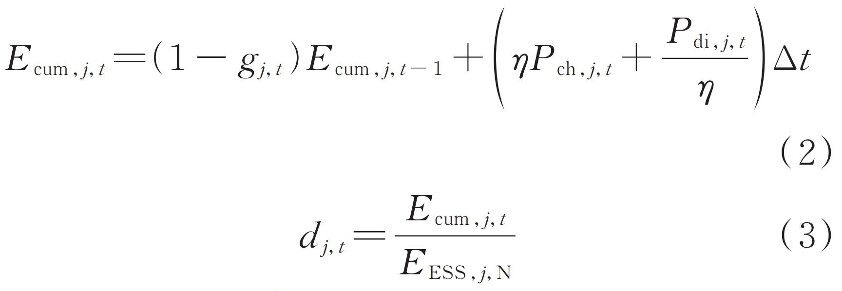
In the formula: Ecum, j, t are the cumulative energy consumption of the grid connected energy storage system at the jth node during the t period in a continuous charging or discharging state; Dj, t is the discharge depth of the grid connected energy storage system at the jth node in time period t; Pch, j, t and Pdi, j, t are the impulse and discharge power of the grid connected energy storage system at the jth node during the t period, respectively; η Charge and discharge efficiency for energy storage; Δ T is the statistical time interval, taken as 1 hour; EESS, j, N are the rated capacity of the jth node grid connected energy storage system.
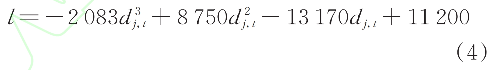
Then, curve fitting is performed on the data of the energy storage discharge depth measured by the rain flow counting method and its corresponding cycle usage times. Typically, a third-order polynomial function is used to characterize the relationship between the cycle usage times l and the discharge depth dj, where t is expressed as:
To calculate the number of cycle charging and discharging times corresponding to different discharge depths during the actual operation of the energy storage system, it is necessary to unify l to the 100% discharge depth scale, as shown in equation (5), and then calculate the cumulative cycle times of the energy storage system on a typical day, as shown in equation (6).
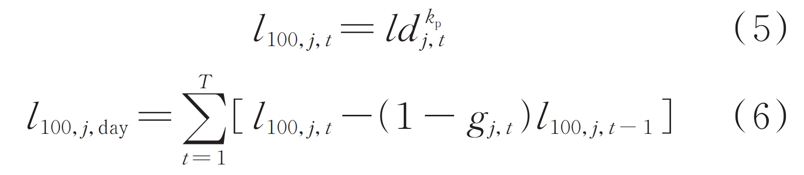
In the formula: l100, j, t are the equivalent number of cycles of the grid connected energy storage system at the jth node of time period t at 100% discharge depth; Kp is the constant obtained by fitting, and different types of energy storage have different values; L100, j, day is the typical daily cumulative total number of cycles for the jth node grid connected energy storage system; T is the number of time periods.
According to the typical daily charging and discharging behavior of energy storage, the cycle life of the energy storage system can be obtained as shown in equation (7). In addition, the daily operation and maintenance cost during the cycle life cycle is calculated as shown in equation (8).
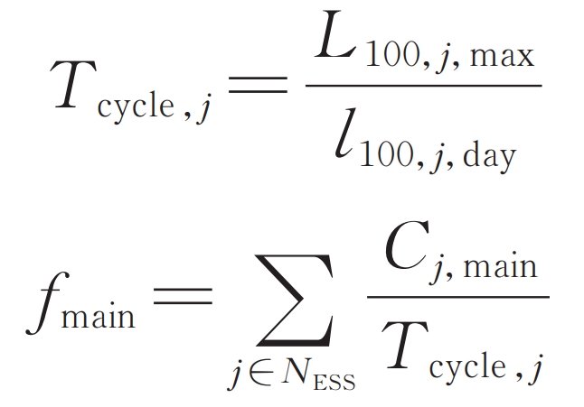
In the formula: Tcycle, j is the cycle life of the jth node grid connected energy storage system; L100, j, max are the maximum charging and discharging times of the grid connected energy storage system at the jth node at 100% discharge depth; Fmain is the daily operation and maintenance cost of energy storage; Cj, main is the total cost of maintenance for each power outage of the jth node’s grid connected energy storage system; NESS is a collection of energy storage grid connected nodes.
1.2 Peak shaving compensation direct benefits
Energy storage participates in peak shaving auxiliary service market transactions, and the discharged electricity is settled according to a certain peak shaving compensation electricity price.
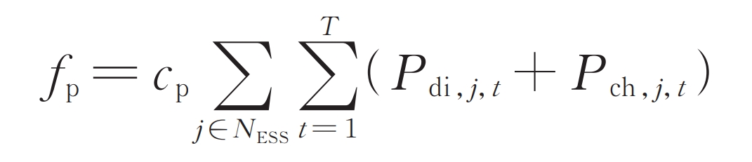
In the formula: fp is the compensation income for the annual peak shaving price of energy storage; CP is the peak shaving compensation electricity price specified in the contract.
2.Robust optimization operation model for flexible distribution network distribution
2.1 Two stage optimization objective function
This article considers the capital of the power grid and the capital of various third-party investment entities for energy storage as a whole, and maximizes the total social capital, i.e. the total operating efficiency of the system. This includes four parts: the electricity sales revenue on the grid side, the cost of purchasing electricity from the higher-level grid, the peak shaving revenue on the energy storage side, and the daily average operation and maintenance cost within its life cycle. Adopting a two-stage distributed robust optimization method based on data-driven approach, effectively handling uncertain factors while ensuring the model has a certain degree of robustness. In the first stage, deterministic optimization is carried out under the known probability distribution of photovoltaic output, and various operating variables of the system are determined and transmitted to the second stage as known quantities; In the second stage, the worst scenario is searched for in the fuzzy set of photovoltaic output probability distribution, and this discrete probability distribution is transmitted to the first stage. Two stages alternate and iterate until convergence, specifically modeled as:
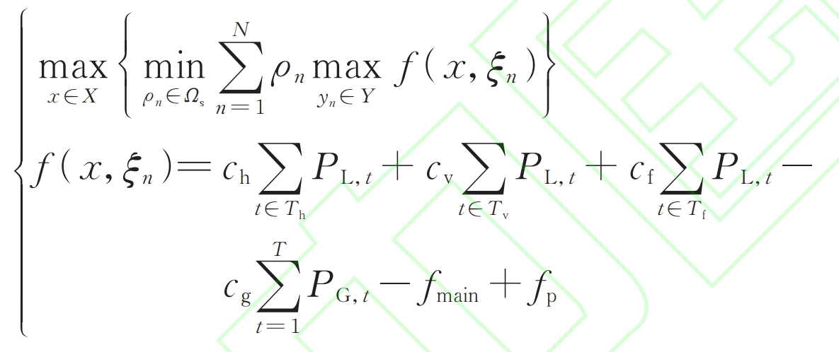
In the formula, x and yn are the decision variables for stage 1 and stage 2 in the nth scenario, respectively. x includes the peak, valley, and normal load power and electricity price, energy storage charging and discharging power, and the electricity purchased from the superior power grid after DR, while yn represents the electricity purchased from the superior power grid; N is the number of scenes; ρ N is the probability corresponding to the scattered field scenario n, which is an uncertain variable; X and Y are the feasible domain sets of x and yn, respectively; Ω ς For ρ N satisfies a fuzzy set; ξ N is the photovoltaic output discrete scenario obtained based on data-driven clustering; C h, c v, and c f are the peak, valley, and average electricity prices after load DR, respectively; Th, Tv, and Tf are the sets of peak, valley, and normal segments, respectively; P L, t is the total system load after DR during period t; Cg is the electricity price for purchasing electricity from the superior power grid; P G, t is the amount of electricity purchased from the superior power grid during time t.
2.2 PV output probability distribution fuzzy set constraints
2.2 1 adjustable KL divergence
Adjustable relative entropy, also known as adjustable KL divergence, can measure the distance between two random distribution functions, and the KL divergence shown in equation (11) Φ Improvement based on KL, as shown in equation (12), adjustable KL divergence Φ Due to its boundedness and symmetry, ADKL is suitable as a constraint metric for fuzzy sets.
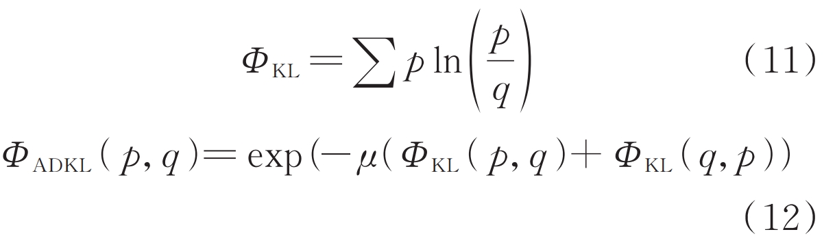
In the formula, p and q are any two discrete probability distributions, respectively; μ Is the sensitivity coefficient, which is taken as 0.5 in this article; Φ ADKL (p, q) ∈ (0,1). The closer the random distribution distance or the higher the similarity, the closer the adjustable KL divergence is to 1. When p=q, Φ ADKL (p, q)=1; On the contrary, the adjustable KL divergence is closer to 0. Therefore, compared to the unbounded nature of traditional KL divergence, the selection of error thresholds for adjustable KL divergence is more explanatory.
2.2 2. Probability distribution fuzzy sets based on adjustable KL divergence
Taking the t0 period as an example to illustrate the specific process of constructing probability distribution fuzzy sets using adjustable KL divergence based on data-driven approach.
1) Collect samples of unit capacity photovoltaic annual output during the t0 period, and cluster the output scenarios as follows Γ T’0={ ξ T’0, 1, ξ T’0, 2, ξ T’0, w, ξ T’0, N}, ξ T’0, w is the wth output discrete scenario, and the corresponding sample frequency is ρ T0, w, the probability set corresponding to each scenario is ς T0={ ρ T0, 1, ρ T0, 2, ρ T0, w, ρ T0, N} as the reference probability distribution, the photovoltaic output PPV during the t0 period can be uniquely determined by the output scenario and its probability distribution.
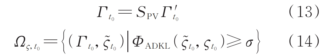
2) If the photovoltaic output is proportional to the capacity, the output scenario of any capacity photovoltaic is shown in equation (13), and its probability distribution satisfies the fuzzy set constraint shown in equation (14).
In the equation: Γ T0 is the output scenario of photovoltaic and unit capacity photovoltaic during the t0 period; SPV is the photovoltaic capacity; Ω ς, T0 is the fuzzy set that satisfies the discrete probabilities of each photovoltaic output scenario during the t0 period; ς͂ T0 and ς T0 represents the actual probability distribution and reference probability distribution of the photovoltaic system, respectively; σ For ς͂ T0 and ς The error threshold between t0, with a value range of (0,1).
In summary, the fuzzy set of photovoltaic output probability distribution constrained by adjustable KL divergence can not only consider historical actual distribution information, but also construct a flexible and adjustable fluctuation range of error threshold, overcoming the blindness of random programming and the conservatism of robust optimization.
2.3 Requirement Response Constraints
In the power system, most users are unable to adjust their electricity demand on a large scale based on dynamic electricity prices, and follow the fixed electricity prices set by the power grid company. A small number of users can adjust their electricity load based on incentives or electricity prices. This article divides the initial power curve of flexible loads in the system into three periods: peak, valley, and flat, and sets up a DR based on electricity price guidance. The power and electricity price of the flexible load before and after response meet equations (15) to (19).
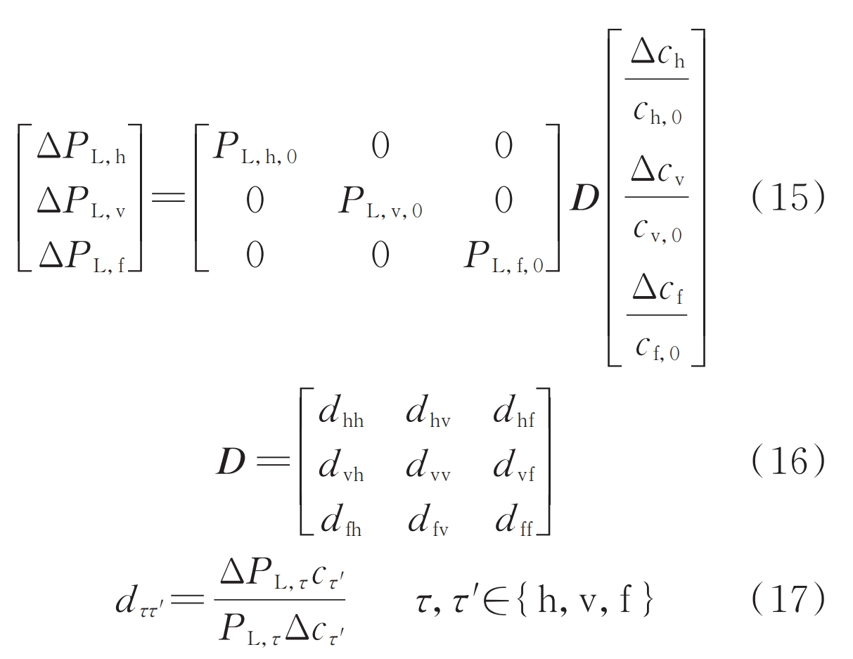
In the formula, the subscripts h, v, and f represent the peak, valley, and flat time periods of the load, respectively; Δ P L, h Δ P L, v Δ P L, f and Δ C h Δ C v Δ CF represents the changes in flexible load and electricity price before and after peak, valley, and normal response periods; P L, h, 0, P L, v, 0, P L, f, 0 and c h, 0, c v, 0, f, 0 are the loads and electricity prices in response to the peak, valley, and normal periods, respectively; D is the elasticity coefficient matrix, where the element d in D ττ ‘ Subscript retrieval of τ = τ ‘ And τ ≠ τ ‘ When is the coefficient of self elasticity and the coefficient of mutual elasticity, respectively. According to literature [23], d ττ ∈ [-0.12, -0.18], d ττ ‘∈ [0.03, 0.10].
There is a linear relationship between load power and electricity price as shown in equation (18), so equation (17) can be transformed into equation (19).
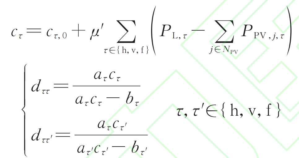
In the equation: c τ, 0 is τ The initial electricity price during the time period; PPV, j, τ For τ The active output of the grid connected photovoltaic system at the jth node of the time period; A τ And b τ Respectively τ Load power P L during the time period, τ And electricity price c τ The coefficient of the linear relationship; μ’ Is a constant; NPV is a collection of photovoltaic grid connected nodes.
2.4 Other constraints
The optimization operation model proposed in the article considers the power flow constraints of AC, DC, and voltage source converters (VSCs), the operation and configuration constraints of ESS and renewable energy, and safety constraints.
3.Convex relaxation processing of the model
The objective function of the aforementioned model includes a bilinear term that multiplies the two continuous variables of electricity quantity and electricity price, and both the energy storage cycle life constraint and power flow constraint contain nonlinear terms. This makes the original flexible distribution network distribution robust optimization operation model a mixed integer nonlinear programming (MINLP) problem, which is one of the most difficult problems to solve in the planning field, It belongs to the (non deterministic polynomials, NP) – difficult problem. If commonly used MINLP solvers such as the simplified branch and bound (SBB) method are used directly to solve, the computational speed is slow and the optimal solution of the optimization problem is often not obtained. To facilitate the use of mature commercial solvers, it is necessary to perform line convexity on the model before using the C&CG algorithm for solution.
3.1 Equivalent Mathematical Transformation Method
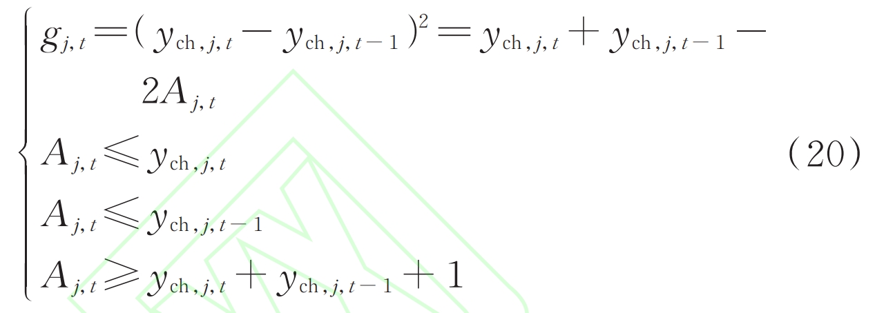
After the expansion of equation (1), there is a term containing the multiplication of binary variables ych, j, t of adjacent charging states. The auxiliary variables Aj, t=ych, j, t ych, j, t-1 are introduced, and the equivalent mathematical transformation is transformed into the linear inequality constraint shown in equation (20).
3.2 Big M Method
In equation (6), the constraint on the number of cumulative cycles of energy storage is calculated, including the product term of binary variables gj, t and continuous variables l100, j, t-1. The auxiliary variable Bj is introduced, t=l100, j, t-1 gj, t to convert equation (6) into a linear constraint, and a new constraint term is added using the large M method, as shown in equation (21).
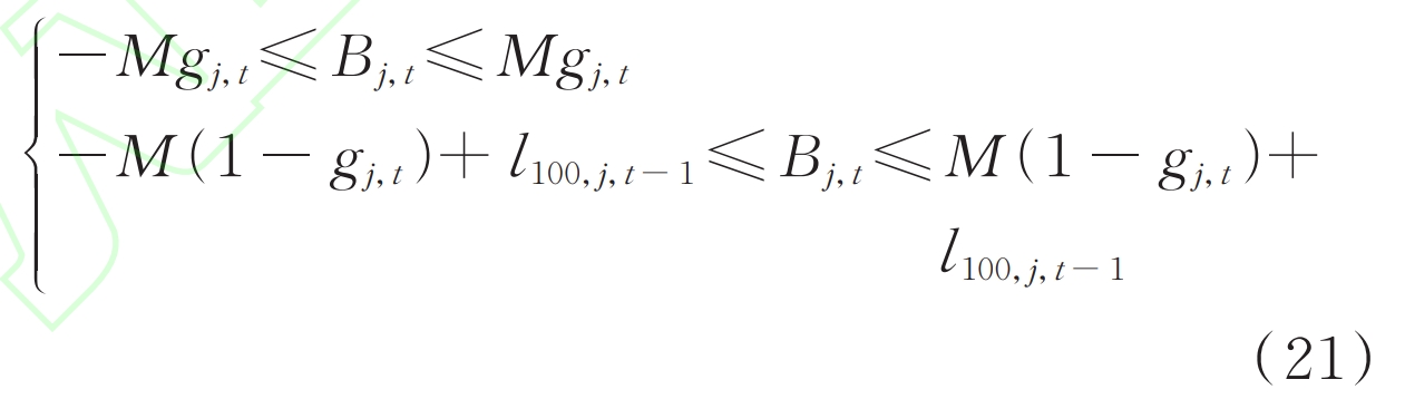
In the equation, M is a constant that is several orders of magnitude larger than the continuous variables l100, j, t-1.
3.3 Convex envelope method
The objective function equation (10) includes the product term of electricity quantity and electricity price after DR, the DC power flow constraint equation Appendix A (A7) and equation (A8) contain both the primary and square terms of DC current, the AC power flow constraint equation (A5) and VSC modulation voltage relationship equation (A9) contain both the primary and square terms of voltage at node C within VSC, and the modulation ratio and DC voltage multiplication term in equation (A9), Both can be regarded as bilinear terms and can be convex treated using the McCormick method (also known as the convex envelope method). Among them, the multiplication of the two continuous variables in equation (10) and equation (A9) adopts M-envelope, and auxiliary variable C is introduced τ = C τ P L, τ And the auxiliary variables Dj, t=MvUDC, j, t, are added with constraints (22) and (23), where Mv is the modulation ratio, with a value range of [0.8, 1.0], and UDC, j, t are the DC voltage of the jth node in time period t. The square term of DC current and VSC internal node voltage is processed using T envelope, as shown in equations (24) and (25).
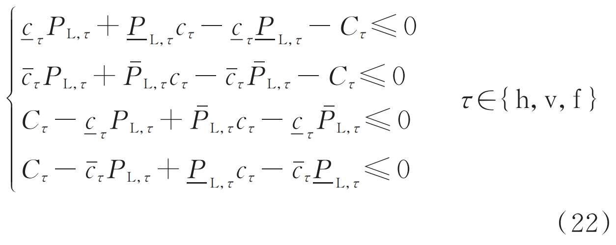
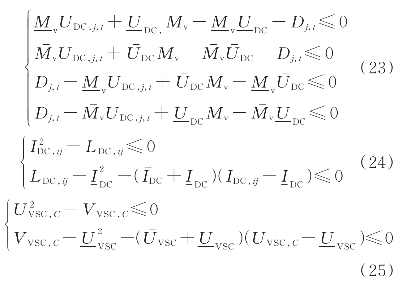
In the equation: c ˉτ、- C τ And P ˉ L, τ、- P L, τ Respectively τ The upper and lower limits of the electricity price and load power during the time period; M ˉ v. – M v and U ˉ DC and – U DC are the upper and lower limits of modulation ratio Mv and DC voltage, respectively; IDC, ij is the current flowing through branch ij; UVSC, C and VVSC, where C is the voltage and the square of the voltage at node C within the VSC; I ˉ DC, – I DC, and U ˉ VSC and – U VSC are the upper and lower limits of DC current and voltage of internal node C in VSC, respectively.
3.4 Second order cone convex relaxation method
In AC power flow, equation (A5) in Appendix A is a quadratic non convex constraint, which is calculated using second-order cone convex relaxation, as shown in equation (26).

In the formula: Pij, t, Qij, t are the active and reactive power of branch ij during time t; Vj, t is the square of the voltage of the jth node in time period t; Lij, t is the load of branch ij during time t.
In summary, according to sections 3.1 to 3.4, the original MINLP model can be transformed into an easy to handle mixed integer convex programming (MICP) problem, which can be efficiently solved by calling mature commercial solvers such as Gurobi.
4.C&CG solving algorithm
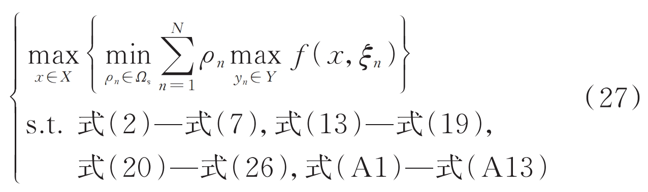
Establish a two-stage distributed robust optimization model as shown in equation (27), and use the C&CG algorithm to decompose the main problem and sub problems for solution.
4.1 Subproblem
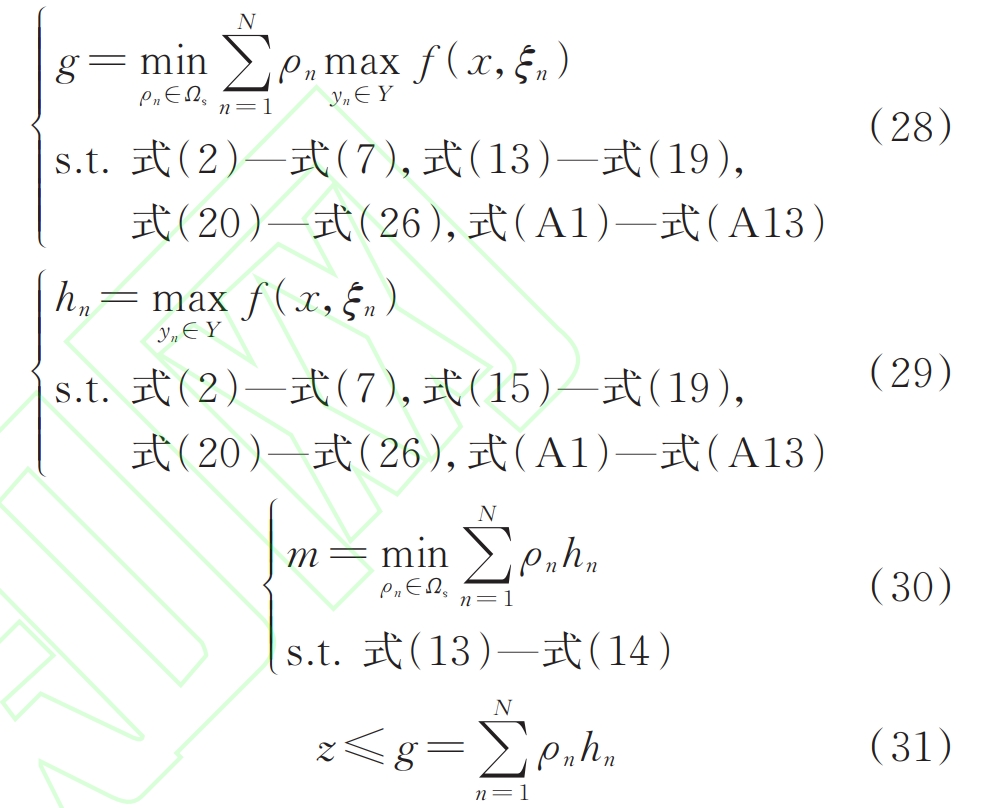
The sub problem is the min max bilevel optimization problem shown in equation (28), aimed at finding the worst-case probability distribution corresponding to N discrete photovoltaic output scenarios that minimize the total operating efficiency of the system. Among them, the decision variables of the inner max model do not include the uncertain probability variables of the outer layer, so the double layer can be decomposed into equations (29) and (30), and solved layer by layer. According to the operating conditions of the flexible distribution network transmitted by the main problem, equation (29) is used to calculate the photovoltaic output scenarios ξ The maximum benefit hn of the system corresponding to n. Equation (30) is used to determine the set of photovoltaic probability distributions that minimize the total system benefits at this time, and is transmitted to the main problem. Based on the optimal objective function g of the subproblem at this time, a new constraint equation (31) is added as the convergence condition of the main problem. In addition, the ESS operation variables involving multi time period coupling have been determined by the main problem as the first stage decision variables, while the N photovoltaic output scenarios in the second stage optimization variables do not consider the time coupling relationship, and can be solved separately for each scenario to reduce the complexity of the solution.
4.2 Main problem
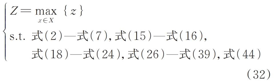
The worst case probability distribution of photovoltaic output, which is an uncertain variable transmitted by the subproblem, is taken as a known quantity. The main problem performs deterministic optimization on the flexible distribution network, as shown in equation (32). The optimal solution Z is solved, and the first stage operating variables are transmitted to the subproblem.
4.3 C&CG algorithm solving process
The steps for solving the max min max two-stage three-layer distributed robust optimization model using the C&CG algorithm are as follows, and the flowchart is shown in Figure A2 of Appendix A.
Step 1: Set the initial lower bound L (0) B to – ∞, and the initial upper bound U (0) B to+∞. Initialize its reference distribution based on historical photovoltaic output data and cluster it to obtain photovoltaic output scenarios ξ N.
Step 2: Start iteration with k (k=0, 1, 2,…), solve the main problem, obtain the optimal solution Z (k) and initial value of the decision variable for the k-th iteration, update the lower bound value L (k) B=max {L (k-1) B, Z (k)} for the k-th iteration.
Step 3: Based on the decision variables transmitted by the main problem, including the peak, valley, and normal load power and electricity price after DR, energy storage charging and discharging power, and superior power grid purchasing power. Solve the subproblem to obtain the worst probability distribution of photovoltaic for the k-th iteration ς͂ (k) t and the optimal solution of the subproblem objective function g (k), update the upper bound value U (k) B=min {U (k-1) B, g (k)} for the k-th iteration.
Step 4: When UB-LB< ε Or ς͂ (k) t= ς͂ (k-1) t, stop iteration, output the optimal running plan, where, ε Is the threshold; On the contrary, the extreme scenario of renewable energy output obtained from solving the k-th subproblem will be ς͂ (k) Transfer t to the main problem, k=k+1, return to step 2.
5.Energy storage operation cost allocation
When multiple energy storage systems collaborate in a flexible distribution network, they work together to balance the fluctuations in renewable energy output and improve the absorption capacity of new energy. The benefits generated should be shared among multiple energy storage systems. The Shapley value method is a commonly used benefit allocation method in cooperative game models. This article applies the improved Shapley value method to multiple energy storage benefit allocation problems, sharing the peak shaving and frequency modulation benefits of each energy storage.
5.1 Shapley value method
The Shapley value method is based on the marginal contribution of each member to the overall goal of the alliance for profit allocation among alliance members. It not only avoids egalitarianism, but also has more rationality and fairness compared to allocation based solely on resource input, allocation efficiency, or a combination of the two. It also reflects the game process of members. The specific calculation process is as follows:
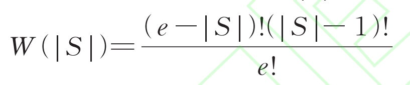
The set N (e1, 2,…, e) represents the e energy storage units that can participate in alliance S, and | S | represents the number of energy storage units included in alliance S. Therefore, the probability of each storage unit forming alliance S during random cooperative operation W (| S |) is:
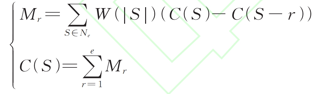
Let M (M1, M2,…, Me) represent the allocation strategy of a cooperative game, assuming that the r th energy storage in the set Ne should be allocated from the total benefit C (S) of alliance S. Mr. satisfies equation (34).
In the formula, C (S – r) represents the total benefit of the distribution network after removing the r-th ESS.
5.2 Improved Shapley value method considering photovoltaic utilization rate
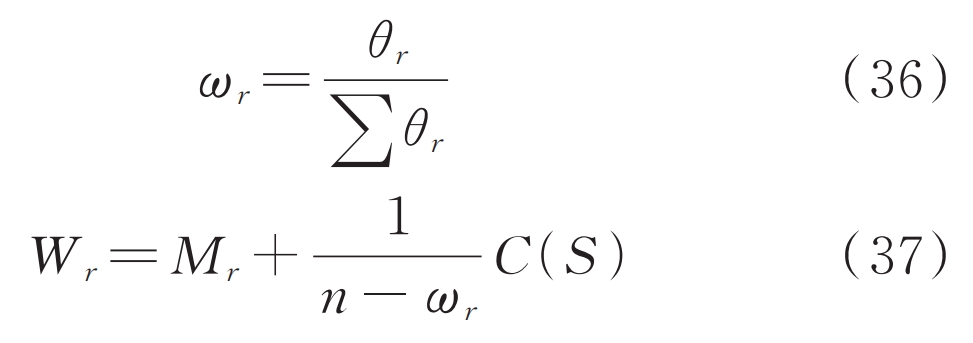
When using the traditional Shapley value method to allocate energy storage benefits, individual differences such as geographical location and specifications of energy storage are not considered, which essentially implies the assumption that the peak shaving effect of each energy storage is 1/n. Therefore, for situations where the peak shaving effect of energy storage is unequal or there are significant differences, it is necessary to make modifications to the benefit allocation scheme of the Shapley value method based on the degree of peak shaving. The utilization rate of renewable energy can reflect the self balancing ability of the distribution network and reflect the degree of utilization of renewable energy under the role of energy storage and allocation. Assuming that the renewable energy utilization rate of the system when the r-th energy storage is acting alone is θ R is:
In the formula: EPV represents the typical daily power generation of each photovoltaic system; EL is the total daily load of the system.
New weight for the r-th energy storage ω As shown in equation (36), use ω The result of obtaining the r th energy storage allocation benefit Wr is shown in equation (37).
6.Example analysis
6.1 Example data
The article takes a 293 node flexible distribution network as an example for analysis, as shown in Figure B1 of Appendix B. The system consists of 12 10 kV feeders and 8 VSCs, with the DC part shown in the dashed box in the figure. The photovoltaic data in the article is the actual historical data collected from a certain area in Nansha District, Guangzhou City, China, on the basis of one year’s illumination intensity and environmental temperature. Based on data-driven data, the discrete probability distribution histogram of photovoltaic daily output is shown in Figure B2, the typical photovoltaic output curve is shown in Figure B3, and the typical system load curve is shown in Figure B4. The grid connection position and capacity of photovoltaic power plants, energy storage systems, and other parameter values in the optimization model are shown in Table B1, and the upper and lower limits of each variable value are not displayed. In the initial electricity price reference, the self elasticity coefficient is -0.15 and the mutual elasticity coefficient is 0.03 in the demand response constraint. Convergence criterion constant in C&CG algorithm κ It is 10 − 6. The GAMS software version used for optimization calculation is 24.5.6. The hardware environment is Intel Xeon CPU E3-1270 3.50 GHz, with 16 GB of memory.
6.2 Result analysis
To verify the effectiveness of the method proposed in this article, the following calculation scenario is set up to compare and analyze the impact of demand response and energy storage cycle life on operating results.
Scenario 1: Without considering demand response and energy storage cycle life model, utilizing distributed robust optimization to run the model.
Scenario 2: Consider demand response without considering the energy storage cycle life model, and use distributed robust optimization to run the model.
Scenario 3: Without considering demand response, consider the energy storage cycle life model, and use distributed robust optimization to run the model.
Scenario 4: Simultaneously considering demand response and energy storage cycle life model, utilizing distributed robust optimization to run the model. The adjustable KL divergence threshold is 0.5.
Scenario 5: Simultaneously considering demand response and energy storage cycle life models, utilizing traditional robust optimization to run the model. The uncertainty threshold of the box type is ± 0.5.
Scenario 6: Simultaneously considering demand response and energy storage cycle life models, utilizing deterministic optimization to operate the model.
Scenario 7: Simultaneously considering demand response and energy storage cycle life model, utilizing distributed robust optimization to run the model. The model is not convex and solved using the SBB solver, with an adjustable KL divergence threshold of 0.5.
The optimization results under different scenarios are shown in Table 1.
| Scene | Electricity sales revenue/(10000 yuan · day ^ -1) | Electricity purchase cost/(10000 yuan per day ^ -1) | Peak shaving efficiency of energy storage/(10000 yuan · day ^ -1) | Energy storage system operation and maintenance cost/(10000 yuan · day ^ -1) | Total benefit/(10000 yuan · day ^ -1) | Solution time/s |
| 1 | 268.651 | 64.323 | 2.401 | 0.200 | 206.529 | 558.5 |
| 2 | 207.991 | 65.545 | 2.222 | 0.200 | 144.468 | 625.3 |
| 3 | 268.651 | 62.360 | 3.589 | 0.328 | 209.551 | 584.7 |
| 4 | 207.991 | 62.700 | 3.516 | 0.390 | 148.417 | 739.6 |
| 5 | 207.991 | 64.932 | 3.223 | 0.241 | 144.578 | 230.0 |
| 6 | 207.991 | 58.919 | 1.519 | 0.207 | 150.383 | 78.8 |
| 7 | 201.454 | 64.276 | 3.339 | 0.362 | 140.155 | 3 186.3 |
6.2 1. The impact of demand response on system optimization operation
Scenario 2 and Scenario 4 both guide users to optimize the load curve through demand response based on time-of-use electricity price incentives. Taking Scenario 4 as an example, the load curve before and after demand response is shown in Figure B5 in Appendix B. Comparing the operating results under Scenarios 1 and 2, as well as Scenarios 3 and 4 in Table 1, it can be seen that when the system considers demand response and transfers the electricity consumption behavior of the peak electricity price to the valley value, it sacrifices 29.16% of the electricity sales revenue, thereby reducing the load peak valley difference and improving power supply reliability. At the same time, considering demand response, the peak shaving benefits of energy storage decreased by 8.06% and 2.06% respectively, which to some extent alleviated the peak shaving pressure of energy storage. In summary, the demand response based on electricity price incentives in this article can be used as one of the methods for system peak shaving and valley filling, with good regulatory ability, and the effect will become more apparent as the flexible load participating in demand response increases. However, the peak shaving effect of energy storage regulation on photovoltaic power generation has weakened, as the matching degree between the response load curve and photovoltaic output curve has decreased, resulting in an increase in the light rejection rate. This is reflected in an increase of 1.90% and 0.54% in the purchasing cost of the system from the higher-level power grid, respectively. Therefore, in future research, further consideration can be given to demand response based on penalty incentives for light abandonment, guiding users’ electricity consumption behavior to shift to the peak period of new energy output, in order to promote the integration and consumption of new energy into the grid.
6.2 2. The impact of energy storage cycle life on system optimization operation
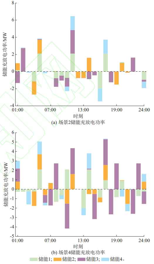
Compare scenarios 1 and 3, as well as scenarios 2 and 4, only considering the energy storage cycle life model. Among them, the energy storage life in scenarios 1 and 2 is set to 1000 days, and the energy storage life under each scenario is shown in Table B2 of Appendix B. Based on Table 1, it can be seen that considering the energy storage cycle life model is beneficial for improving the peak shaving efficiency of energy storage. However, the increase in the number of charging and discharging state transitions leads to a shortened lifespan of energy storage and an increase in the daily operation and maintenance cost of energy storage. However, the increase in peak shaving benefits for energy storage is still greater than the increased operation and maintenance costs, and the overall efficiency of the system has improved. Analyze the impact of the energy storage cycle life model on its own peak shaving effect. Taking Scenarios 2 and 4 as examples, the comparison of energy storage charging and discharging quantities is shown in Figure 1. Analysis shows that compared to Scenario 2, Scenario 4 significantly improves the depth of energy storage charge and discharge and the number of state transitions. In summary, compared to traditional optimization models that consider the energy storage life to be a constant, the energy storage life model established in this article more accurately reflects the actual operating conditions of energy storage. When optimizing the operation of the system, considering the impact of energy storage charging and discharging on life loss can maximize the comprehensive benefits of the system in the game process of energy storage operation and maintenance costs and peak shaving benefits.
6.2 3. The impact of optimization methods on system optimization operation
To verify the effectiveness of the distributed robust optimization method in this article, scenarios 4, 5, and 6 respectively utilized distributed robust, traditional robust, and deterministic methods to optimize the operation of the examples in this article. The cost indicators are shown in Table 1. Analysis shows that all three schemes consider load demand response and energy storage life models, and the sales benefits are equal to 2.07991 million yuan/day, while the distribution robust optimization results of the total benefits are between deterministic and robust methods. This is because Scenario 4 and 5 respectively use distributed robust and robust models to search for extreme photovoltaic output scenarios or scenario probability distributions that minimize comprehensive income. Compared to deterministic optimization, both of them improve the robustness of the system under uncertain conditions, that is, improve operational flexibility and safety at the expense of certain economic benefits. Compared to scenarios 4 and 5, traditional robustness sets a box uncertainty interval for photovoltaic output without incorporating its probability distribution characteristics. The distributed robust method is based on the statistical data of photovoltaic output to obtain distribution information, and uses adjustable KL divergence to construct its fuzzy set constraints, searching for extreme probability distributions, effectively improving the shortcomings of traditional robust box intervals that are too conservative. In summary, distributed robustness balances economy and robustness to a certain extent, and is more advantageous when applied to the optimization operation of power grids with uncertain factors. In addition, in Scenario 4, after optimizing using the model proposed in this article, the AC and DC subnets exchange power through VSC, as shown in Figure B6 in Appendix B. The AC system supplies power to the DC subnet through VSC, or peak shaving electricity is provided by the energy storage inside the DC subnet.
6.2 4. The impact of adjustable KL divergence threshold on system optimization operation
According to section 2.2, adjustable KL divergence threshold σ The value range is (0, 1). By adjusting σ The fuzzy set constraint between the actual probability distribution of photovoltaic and the reference distribution can be changed, which may alter the worst-case output probability scenario sought. Different σ The robust optimization results of distribution under values are shown in Table B3 of Appendix B. In the σ In the process of changing from small to large, the overall efficiency of the system gradually improves, and the results of distributed robust optimization are always between robust and deterministic optimization methods. σ The closer to 0, the greater the error level between the probability distribution fuzzy set constructed by adjustable KL divergence and the sample set driven by data, and the closer the optimization results are to traditional robustness; σ The closer to 1, the smaller the distance constraint between the fuzzy set and the sample set, and the higher the coincidence degree, that is, the photovoltaic output fluctuation range is constrained near the typical probability distribution. At this point, the results of distributed robust optimization are closer to deterministic optimization. In summary, by changing the threshold of adjustable KL divergence, it is possible to constrain the upper and lower bounds of the fuzzy set for the fluctuation range of uncertain variables, placing the distribution robust optimization configuration result between deterministic optimization and traditional robust optimization. The configuration scheme takes into account a certain degree of economy and robustness.
6.2 5. The impact of convex processing methods on system optimization operation
To highlight the effectiveness of the convexity processing method proposed in this article, the solution ability and accuracy of solving mixed second-order cone programming problems using the Gurobi solver and solving MINLP problems using the SBB solver were compared with scenario 4 and 7 in Table 1. It can be seen that both models can be solved, but after being processed by the various convexity methods proposed in this article, all indicators in the total benefit objective function of the system are better than those of the non convexity treated model, and the efficiency is increased by 5.89%. This indicates that convexity processing can increase the optimization space of the model, enabling the system to find more optimal solutions. In addition, the solving time of the SBB solver is 4.3 times that of the Gurobi solver, which is not advisable for optimization problems, especially scheduling problems, in large-scale systems. In summary, the convexity method proposed in this article can effectively improve the optimization ability and solving efficiency of the model.
6.2 6. Model performance comparison
To analyze the efficiency of the optimization model in different scenarios in this article, compare the system optimization solution time of Scenario 1 and Scenario 2, 3, and 4 in Table 1. When using distributed robust methods to solve, embedding demand response and energy storage cycle life separately or simultaneously can increase the solution time by 66.8-181.1 seconds, which is within an acceptable range. However, both are beneficial for peak shaving and valley filling in flexible distribution networks, and more accurately reflect the operating conditions of the system. Therefore, demand response and energy storage cycle life constraints should be included in the optimization operation model; Compared to scenarios 4, 5, and 6, the model considers both demand response and energy storage cycle life constraints. The two-stage distributed robust optimization method has a solution time of 509.3 seconds longer than the robust method. This is because traditional robustness only uses box uncertainty intervals to represent photovoltaic output uncertainty, without considering its true probability distribution; Compared to the deterministic optimization method, this is 660.8 seconds longer because the deterministic method does not consider the fluctuation uncertainty of photovoltaic output and does not have a two-stage iterative optimization process, resulting in a higher operational risk for the decision plan. Therefore, to ensure that the decision-making scheme has a certain degree of robustness under photovoltaic output fluctuations, and to ensure the safe and reliable operation of the system, a two-stage distributed robust optimization method should be adopted. In summary, the model constructed in this article takes into account demand response constraints and energy storage life constraints, and adopts distributed robust optimization method to solve, aiming to make the model more in line with the actual operating conditions of the power system and effectively improve the operational reliability of the decision-making scheme. Although the solution time is relatively extended, it is within an acceptable range.
6.2 7. Allocation of energy storage peak shaving benefits
According to Chapter 4, the marginal benefits of each energy storage participating in peak shaving are first obtained.
According to equations (46) and (47), calculate the peak shaving benefit Mi based on the Shapley value method when each energy storage works together, and calculate the photovoltaic utilization index and the improved Shapley value method allocation result Wi when each energy storage works separately, as shown in Table 2.
| Energy storage number | Shapley value method for sharing benefits Mi/yuan | Voltage utilization rate under single action/% | Improved Shapley Value Method for Sharing Benefits Wi/Yuan |
| 1 | 7 487.86 | 36.24 | 8 156.08 |
| 2 | 6 061.58 | 28.30 | 4 657.27 |
| 3 | 18 575.80 | 46.36 | 1 885.58 |
| 4 | 3 039.84 | 23.82 | 466.15 |
Considering the photovoltaic utilization rate of the system when each energy storage system operates independently, the photovoltaic utilization rate is the highest when the energy storage system operates in 3. In order to encourage it to join multiple energy storage alliances to participate in peak shaving, based on the factor of photovoltaic utilization rate, the allocation weight and value of each energy storage weight are further increased on the basis of equal division. From Table 2, it can be seen that compared to the traditional Shapley value method, the 3-day peak shaving benefit allocation of energy storage system has increased by 3309 yuan. Similarly, energy storage system 1 has increased by 668 yuan, while energy storage system 2 and energy storage system 4 have decreased by 1404 yuan and 2573 yuan, respectively. This indicates that the improved Shapley value method can effectively correct the impact of the difference in the ability of each energy storage participating in system peak shaving on the cost allocation results. The above results not only demonstrate that the method proposed in this paper can achieve optimized operation and cost allocation of multiple energy storage, but also demonstrate that the use of collaborative energy storage has better peak shaving benefits.
7.Conclusion
This article proposes a distributed robust optimization operation method and benefit balancing strategy that takes into account the energy storage cycle life, in response to the insufficient consideration of energy storage life models and peak shaving benefits in the optimization operation of flexible distribution networks. The conclusions obtained are as follows.
1) The demand response of time-of-use electricity price incentives can guide users to optimize the load curve, reduce the load peak valley difference, and reduce the peak shaving pressure of energy storage, improving power supply safety and reliability.
2) The charging and discharging behavior of energy storage affects its cycle life. By embedding an energy storage cycle life model in the optimization operation problem, it can more reasonably optimize the energy storage operation and accurately reflect its operating costs and benefits, and more truly reflect the economic benefits of energy storage.
3) The distributed robust optimization method overcomes the shortcomings of traditional robust methods that are too conservative, and also avoids the operational risks of deterministic optimization schemes under uncertain photovoltaic output factors, improving the robustness and safety of the schemes. Constructing fuzzy set constraints based on adjustable KL divergence to flexibly adjust and balance the economy and robustness of schemes.
4) By using the improved Shapley value method and considering the factors that affect the renewable energy utilization rate of the system, the allocation weights of each energy storage are adjusted to obtain the peak shaving benefits of multi energy storage allocation synergy, and the final peak shaving benefits of each energy storage allocation are calculated, reflecting the fairness of benefit allocation.
However, this article has conducted a study on the collaborative peak shaving benefit sharing among multiple energy storage entities in flexible distribution networks, but has not yet considered the business model of grid capital and third-party investment entities participating in the electricity market. In order to effectively solve the problem of poor investment efficiency in energy storage and promote more participation in the energy market, the next step of work should be based on the idea of compensating third-party investment entities for energy storage by power grid enterprises, and determine the subsidy plan given by power grid companies to various energy storage investors based on game theory, further improving the distribution of benefits among energy storage investment entities.