
The global transition towards a sustainable energy future, driven by carbon neutrality goals, has led to a significant increase in the penetration of renewable energy sources (RES) like photovoltaic (PV) and wind power into power systems. Industrial and commercial parks, as major energy consumption hubs, play a critical role in this transition. Optimizing the energy dispatch within these parks is paramount for achieving energy savings and emission reduction. However, the inherent intermittency and uncertainty of RES, coupled with the fluctuating nature of electrical loads, pose substantial challenges to effective energy management. To address these challenges, the coordinated dispatch of source, grid, load, and storage (SGLS) has emerged as a vital operational paradigm for modern microgrids. By intelligently scheduling power flows among distributed generators, the utility grid, energy storage systems, and loads, this approach aims to satisfy demand while maximizing renewable utilization and minimizing operational costs.
Extensive research has been conducted on SGLS coordination. Initial studies primarily focused on single-objective economic optimization, minimizing electricity purchase costs but often neglecting the degradation of critical assets like energy storage batteries. Subsequent work introduced multi-objective frameworks to balance economy with reliability, employing robust optimization to handle RES uncertainty. Yet, these methods often require manual weighting of objectives, which is difficult to adapt dynamically. More recently, artificial intelligence, particularly deep reinforcement learning, has been applied to learn optimal storage control policies through trial and error. While adaptive, these “black-box” models suffer from a lack of interpretability, which is crucial for operational trust in real-world systems.
Concurrently, modeling the lifetime degradation of energy storage batteries has gained considerable attention. Research has developed aging cost models based on electrochemical principles, quantifying the impact of factors like depth of discharge (DOD) and state-of-charge (SOC) stress. Frameworks have been proposed to schedule batteries by limiting charge/discharge rates and SOC windows to reduce lifespan loss. Methods such as rainflow counting are used to analyze cyclic aging, and metrics like equivalent full cycles serve as lifespan indicators in optimization models. Nevertheless, many of these advanced battery aging models are optimized in isolation and are not fully integrated into the broader energy dispatch framework of a microgrid.
To bridge this gap, this paper proposes a novel bi-level optimization model for SGLS cooperative scheduling. The core innovation lies in the explicit and iterative coordination between system-wide economic dispatch and detailed, health-conscious control of individual energy storage battery units. The upper-level model schedules the aggregate power flow from PV, wind, the grid, and the total storage system to minimize daily electricity costs. The lower-level model then disaggregates the total storage power setpoint into optimal charge/discharge commands for each individual energy storage battery, with the explicit goal of minimizing cumulative lifespan degradation. The lower level feeds back aging information to the upper level, enabling a holistic strategy that balances immediate cost with long-term asset health. This approach overcomes the limitations of single-layer or purely economic models, providing a transparent and efficient scheduling framework for practical park energy management systems.
System Architecture and Mathematical Modeling
The considered park microgrid comprises photovoltaic panels, wind turbines, AC loads, an energy storage cabinet (composed of multiple individual battery units), inverters, and a central dispatch system. The fundamental operating principle is to prioritize renewable generation for supplying loads. Surplus renewable energy charges the energy storage battery cabinet, which subsequently discharges during periods of high grid electricity prices to offset expensive grid purchases. When renewable generation is insufficient, power is drawn from the main grid to ensure supply reliability. The energy storage battery cabinet is charged during low-price (valley) periods to exploit arbitrage opportunities offered by time-of-use (TOU) tariffs.
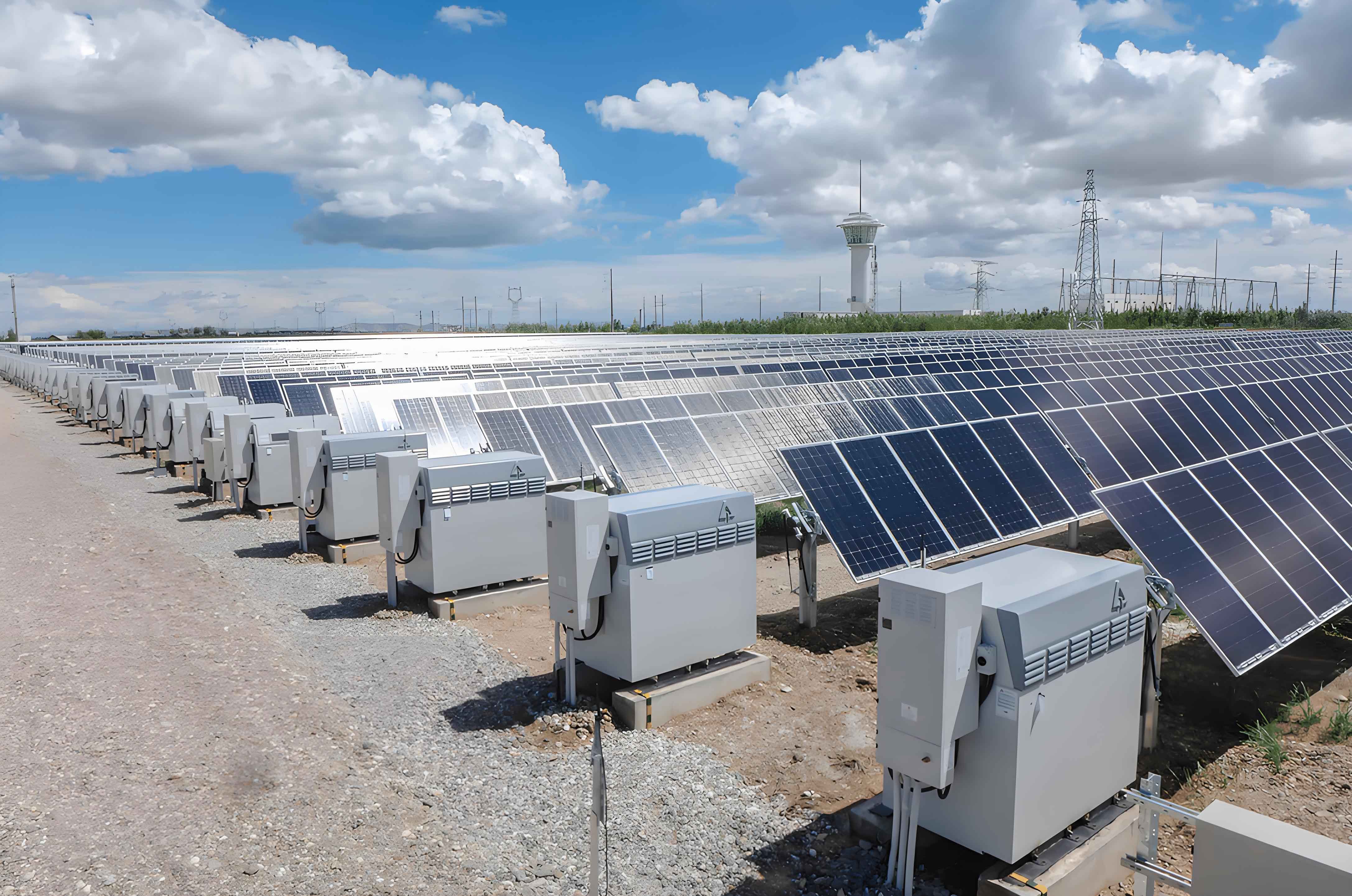
The dispatch of the energy storage battery system is central to this operation. The storage cabinet’s total charge/discharge power is the sum of the power of each constituent energy storage battery, each of which can be controlled independently. The mathematical models for each component are established as follows.
Wind Power Generation Model
Wind turbine output power is a function of wind speed. The input wind power is given by:
$$P_{\text{WT}}^{\text{in}} = \frac{1}{2} \rho A v^3 = \frac{1}{2} \rho \pi R^2 v^3$$
where $\rho$ is air density, $v$ is wind speed, $R$ is rotor blade radius, and $A$ is the swept area. The actual electrical output power is:
$$P^{\text{WT}}_t = C_P \cdot P_{\text{WT}}^{\text{in}} = \frac{1}{2} \rho A v^3 C_P$$
Here, $C_P$ is the power coefficient, and $P^{\text{WT}}_t$ serves as the available wind power input for the upper-level dispatch at time interval $t$.
Photovoltaic Power Generation Model
PV panel output depends primarily on solar irradiance and ambient temperature. The generated power at time $t$ is modeled as:
$$P^{\text{PV}}_t = P_{\text{STC}} \cdot \frac{G_{\text{AC}}}{G_{\text{STC}}} \cdot \left[1 + \delta (T_c – T_r)\right]$$
$$T_c = T_e + 30 \cdot \frac{G_{\text{AC}}}{1000}$$
In these equations, $P^{\text{PV}}_t$ is the PV output power; $P_{\text{STC}}$ is the rated power under standard test conditions (STC); $G_{\text{AC}}$ and $G_{\text{STC}}$ are the actual and STC irradiance levels, respectively; $\delta$ is the temperature coefficient of power; $T_c$, $T_r$, and $T_e$ are the cell, reference (25°C), and ambient temperatures, respectively.
Aggregate Energy Storage System Model
The Energy Storage System (ESS) is crucial for balancing supply and demand. Its aggregate charge/discharge power at time $t$ is denoted as $P^{\text{ESS}}_t$ (positive for discharge, negative for charge). The power is constrained by its rated capacity:
$$-P^{\text{ESS}}_{\text{max,ch}} \leq P^{\text{ESS}}_t \leq P^{\text{ESS}}_{\text{max,dis}}$$
For simplicity, we often assume symmetric limits: $ -P^{\text{ESS}}_{\text{max}} \leq P^{\text{ESS}}_t \leq P^{\text{ESS}}_{\text{max}}$. The State of Charge (SOC) dynamics for the entire cabinet are:
$$
\text{SOC}_{t+1} = \text{SOC}_t + \frac{\Delta t \cdot \eta^{\text{ESS}}_{\text{ch}} \cdot P^{\text{ESS,ch}}_t}{E^{\text{ESS}}} – \frac{\Delta t \cdot P^{\text{ESS,dis}}_t}{\eta^{\text{ESS}}_{\text{dis}} \cdot E^{\text{ESS}}}
$$
where $E^{\text{ESS}}$ is the total energy capacity, $\eta^{\text{ESS}}_{\text{ch}}$ and $\eta^{\text{ESS}}_{\text{dis}}$ are charge and discharge efficiencies, and $\Delta t$ is the duration of a time interval. The SOC must be maintained within safe operating limits:
$$ \text{SOC}_{\text{min}} \leq \text{SOC}_t \leq \text{SOC}_{\text{max}} $$
Lifetime Degradation Model for Individual Energy Storage Batteries
This is a core contribution of the lower-level optimization. The lifespan of an energy storage battery is primarily consumed by cyclic aging, which is accelerated by deep discharge cycles and operation at extreme SOC states. Let $DOD_t$ denote the depth of discharge for a cycle at time $t$. The lifetime loss $\Delta S_t$ for a single energy storage battery during interval $t$ is modeled as a piecewise function considering both DOD stress and SOC stress (operation outside a preferred range, e.g., 30%-80%):
$$
\Delta S_t = \begin{cases}
1 \times 10^{-4} \cdot DOD_t^{50\%} + M_t, & \text{if } DOD_t \leq 50\%, 30\% \leq \text{SOC}_t \leq 80\% \\
1 \times 10^{-4} \cdot DOD_t^{50\%} \cdot (1 + 5\%) + M_t, & \text{if } DOD_t \leq 50\%, \text{SOC}_t < 30\% \text{ or } \text{SOC}_t > 80\% \\
1 \times 10^{-4} + M_t, & \text{if } DOD_t > 50\%, 30\% \leq \text{SOC}_t \leq 80\% \\
1 \times 10^{-4} \cdot (1 + 5\%) + M_t, & \text{if } DOD_t > 50\%, \text{SOC}_t < 30\% \text{ or } \text{SOC}_t > 80\%
\end{cases}
$$
An additional penalty $M_t$ is incurred for switching between charge and discharge states within a short period, as frequent transitions also cause wear:
$$
M_t = \begin{cases}
1 \times 10^{-6}, & \text{if } DOD_t > 0 \text{ and charge/discharge state switches at } t \\
0, & \text{otherwise}
\end{cases}
$$
Assuming an initial battery lifespan of 1 (representing 100%), the remaining lifespan of a single energy storage battery after $n$ intervals is:
$$ S_n = 1 – \sum_{t=1}^{n} \Delta S_t $$
The objective of the lower level is to minimize the sum of $\Delta S_t$ across all batteries and over the scheduling horizon.
Bi-Level Optimization Framework and Solution Methodology
The proposed solution is a coordinated bi-level optimization. The upper level handles system-wide economic dispatch, while the lower level performs health-aware management for each energy storage battery. They interact iteratively to find a globally efficient and sustainable operating point.
Upper-Level Model: Economic Dispatch
Objective Function: The goal is to minimize the total electricity purchase cost from the main grid over a scheduling horizon $T$ (e.g., 24 hours).
$$ \min \sum_{t=1}^{T} C^{\text{MG}}_t \cdot \left( P^{\text{(MG,L)}}_t + P^{\text{(MG,ESS)}}_t \right) $$
Here, $C^{\text{MG}}_t$ is the TOU electricity price (CNY/kWh), $P^{\text{(MG,L)}}_t$ is grid power directly supplying the load, and $P^{\text{(MG,ESS)}}_t$ is grid power used to charge the energy storage battery cabinet.
Decision Variables: The model determines the power split among all sources at each time step.
| Decision Variable | Description |
|---|---|
| $P^{\text{(PV,L)}}_t$ | PV power to Load |
| $P^{\text{(PV,ESS)}}_t$ | PV power to ESS |
| $P^{\text{(WT,L)}}_t$ | Wind power to Load |
| $P^{\text{(WT,ESS)}}_t$ | Wind power to ESS |
| $P^{\text{(ESS,L)}}_t$ | ESS discharge power to Load |
| $P^{\text{(MG,L)}}_t$ | Grid power to Load |
| $P^{\text{(MG,ESS)}}_t$ | Grid power to ESS |
Constraints:
- Power Balance: Load demand $P^L_t$ must be met at all times.
$$ P^{\text{(PV,L)}}_t + P^{\text{(WT,L)}}_t + P^{\text{(ESS,L)}}_t + P^{\text{(MG,L)}}_t = P^L_t, \quad \forall t $$ - Renewable Generation Limits:
$$ P^{\text{(PV,L)}}_t + P^{\text{(PV,ESS)}}_t \leq P^{\text{PV}}_t, \quad \forall t $$
$$ P^{\text{(WT,L)}}_t + P^{\text{(WT,ESS)}}_t \leq P^{\text{WT}}_t, \quad \forall t $$ - ESS Aggregate Power Definition & Limit: The net power for the ESS cabinet is defined by its charging and discharging sources.
$$ P^{\text{ESS}}_t = P^{\text{(ESS,L)}}_t – \left( P^{\text{(PV,ESS)}}_t + P^{\text{(WT,ESS)}}_t + P^{\text{(MG,ESS)}}_t \right) $$
$$ -P^{\text{ESS}}_{\text{max}} \leq P^{\text{ESS}}_t \leq P^{\text{ESS}}_{\text{max}}, \quad \forall t $$
(Here, $P^{\text{ESS}}_t > 0$ indicates net discharge, $<0$ indicates net charge). - ESS SOC Dynamics & Limits:
$$ \text{SOC}_{t+1} = \text{SOC}_t + \frac{\Delta t \cdot \left( P^{\text{(PV,ESS)}}_t + P^{\text{(WT,ESS)}}_t + P^{\text{(MG,ESS)}}_t \right) \cdot \eta_{\text{ch}}}{E^{\text{ESS}}} – \frac{\Delta t \cdot P^{\text{(ESS,L)}}_t}{E^{\text{ESS}} \cdot \eta_{\text{dis}}}, \quad \forall t $$
$$ \text{SOC}_{\text{min}} \leq \text{SOC}_t \leq \text{SOC}_{\text{max}}, \quad \forall t $$
This upper-level problem is a Mixed-Integer Linear Programming (MILP) model, efficiently solvable using commercial solvers like CPLEX.
Lower-Level Model: Battery Health-Aware Dispatch
Objective Function: Given the total ESS power setpoint $P^{\text{ESS}}_t$ from the upper level, the lower level schedules each of the $N$ individual energy storage batteries to minimize total lifespan degradation.
$$ \min \sum_{t=1}^{T} \sum_{i=1}^{N} \Delta S^{\text{battery}}(i, t) $$
where $\Delta S^{\text{battery}}(i, t)$ is the lifetime loss for battery $i$ at time $t$, calculated via the degradation model in Section 1.3.
Decision Variable: The charge/discharge power for each individual energy storage battery $i$ at time $t$, denoted $P^{\text{battery}}(t, i)$. A positive value indicates discharge, negative indicates charge.
Constraints:
- Power Consistency: The sum of all individual battery powers must equal the aggregate ESS power command from the upper level.
$$ \sum_{i=1}^{N} P^{\text{battery}}(t, i) = P^{\text{ESS}}_t, \quad \forall t $$ - Individual Battery Power and SOC Limits:
$$ -P^{\text{battery}}_{\text{max}} \leq P^{\text{battery}}(t, i) \leq P^{\text{battery}}_{\text{max}}, \quad \forall t, i $$
$$ \text{SOC}^{\text{battery}}_{\text{min}} \leq \text{SOC}^{\text{battery}}(t, i) \leq \text{SOC}^{\text{battery}}_{\text{max}}, \quad \forall t, i $$ - Individual Battery SOC Dynamics: Each battery has its own SOC trajectory based on its power $P^{\text{battery}}(t, i)$ and its share of the total capacity $E^{\text{battery}} = E^{\text{ESS}} / N$.
This lower-level problem is a complex, non-linear optimization due to the piecewise degradation model and the discrete switching penalty $M_t$. A Genetic Algorithm (GA) is well-suited to handle this complexity and search for a near-optimal allocation of power among the energy storage battery units.
Coordinated Solution Algorithm
The overall bi-level algorithm proceeds as follows:
- Initialization: Input forecast data for $P^{\text{PV}}_t$, $P^{\text{WT}}_t$, $P^L_t$, and $C^{\text{MG}}_t$. Initialize system parameters and battery states.
- Upper-Level Solve: Solve the MILP economic dispatch model. Obtain the optimal aggregate schedule, including the vector $[P^{\text{ESS}}_t]$ for all $t$.
- Lower-Level Solve: For the given $[P^{\text{ESS}}_t]$, run the GA to find the power allocation $[P^{\text{battery}}(t, i)]$ that minimizes total battery degradation over the horizon.
- Feedback and Iteration (Optional/Advanced): The cumulative degradation cost from the lower level can be monetized (e.g., CNY/kWh of throughput) and fed back to the upper level as an additional cost term associated with using the energy storage battery system. The upper-level problem is then resolved with this updated cost function. This process iterates until convergence, achieving a true joint optimum of economic and battery health objectives.
- Output: Finalize and output the coordinated dispatch strategy for the microgrid.
Case Study and Performance Analysis
A case study based on a typical industrial park in Northeast China is constructed to validate the proposed bi-level framework. The park has a 2 MW wind turbine and 1000 m² of rooftop PV panels. Typical daily profiles for wind/PV generation, load, and TOU price are used.
| Parameter | Value | Description |
|---|---|---|
| $E^{\text{ESS}}$ | 4 MWh | Total storage capacity |
| $P^{\text{ESS}}_{\text{max}}$ | 1 MW | Max charge/discharge power |
| $\text{SOC}_{\text{min}}, \text{SOC}_{\text{max}}$ | 0.1, 0.9 | Allowable SOC range |
| $N$ | 120 | Number of battery units in cabinet |
| $\eta_{\text{ch}}, \eta_{\text{dis}}$ | 0.95, 0.95 | Charge/Discharge efficiency |
| TOU Price (Peak/Flat/Valley) | 1.2 / 0.8 / 0.4 CNY/kWh | Grid electricity tariff |
The proposed Bi-Level Optimization (BLO) model is compared against a traditional Rule-Based, Single-Layer Optimization (RBSO) strategy. The RBSO follows a simple rule: charge the energy storage battery at maximum rate during valley price periods until full, and discharge at maximum rate during peak price periods until the lower SOC limit is reached, prioritizing economic gain without explicit battery health management.
Results and Discussion
1. Economic Performance: The BLO strategy reduces the total daily electricity purchase cost by 8.12% compared to the RBSO strategy. The key reason is intelligent, predictive scheduling. The BLO model, aware of future renewable generation and load patterns, schedules more strategic charging during low-price periods and coordinates discharge with renewable deficits during high-price periods. In contrast, the RBSO may exhaust the energy storage battery early in the peak period, forcing greater reliance on expensive grid power later when renewables are low.
2. Battery Lifespan Management: This is a critical advantage of the BLO framework. Over a simulated 31-day (744-hour) operational period, the total lifespan loss for the entire energy storage battery cabinet (120 units, starting from a combined “life capital” of 120) is quantified.
| Metric | Bi-Level Optimization (BLO) | Rule-Based Single-Layer (RBSO) |
|---|---|---|
| Initial Combined Lifespan | 120.00 | 120.00 |
| Final Combined Lifespan | 119.28 | 118.78 |
| Total Lifespan Loss | 0.72 | 1.22 |
| Relative Reduction in Loss | 41.0% | – |
The BLO model reduces battery aging by 41%. The lower-level GA successfully distributes the total power demand among the individual energy storage batteries in a way that minimizes deep discharge cycles, avoids extreme SOCs, and reduces the frequency of charge/discharge mode switches—all factors captured in the degradation model $\Delta S_t$.
3. Renewable Energy Utilization: The BLO framework also enhances the consumption of local renewable generation. The share of load demand met by PV and wind increases from 40.85% under RBSO to 46.34% under BLO, an improvement of 5.49 percentage points. This is achieved by more effectively using the energy storage battery to store excess renewable production for later use, rather than simply following a rigid price-based charge/discharge rule.
| Performance Indicator | Bi-Level Optimization | Rule-Based Single-Layer | Improvement |
|---|---|---|---|
| Daily Electricity Cost | Base (Lower) | +8.12% Higher | 8.12% Reduction |
| Battery Lifespan Loss (31-day) | 0.72 | 1.22 | 41.0% Reduction |
| Renewable Energy Penetration | 46.34% | 40.85% | 5.49 pp Increase |
Conclusion
This paper presents a novel bi-level optimization framework for the cooperative dispatch of source, grid, load, and storage in renewable-rich microgrids or industrial parks. The model explicitly addresses the critical trade-off between operational economy and the long-term health of the energy storage battery system, an asset whose degradation significantly impacts lifecycle costs and system reliability. The upper level formulates a standard economic dispatch problem as a tractable MILP model. The lower level incorporates a detailed, physics-inspired degradation model for individual energy storage batteries and solves a non-linear optimization problem via GA to minimize lifespan loss for a given aggregate power schedule.
The case study demonstrates the clear superiority of the proposed approach. Compared to a conventional rule-based strategy focused solely on price arbitrage, the bi-level framework achieves a simultaneous reduction in grid electricity costs (8.12%), a substantial decrease in energy storage battery aging (41%), and a higher utilization rate of local photovoltaic and wind power. By enabling this coordinated, health-aware management of the energy storage battery fleet, the proposed method provides a robust, transparent, and economically sound scheduling framework. It offers significant theoretical insight and practical value for the design and operation of next-generation energy management systems aimed at true sustainability and cost-effectiveness.