
1. System Overview
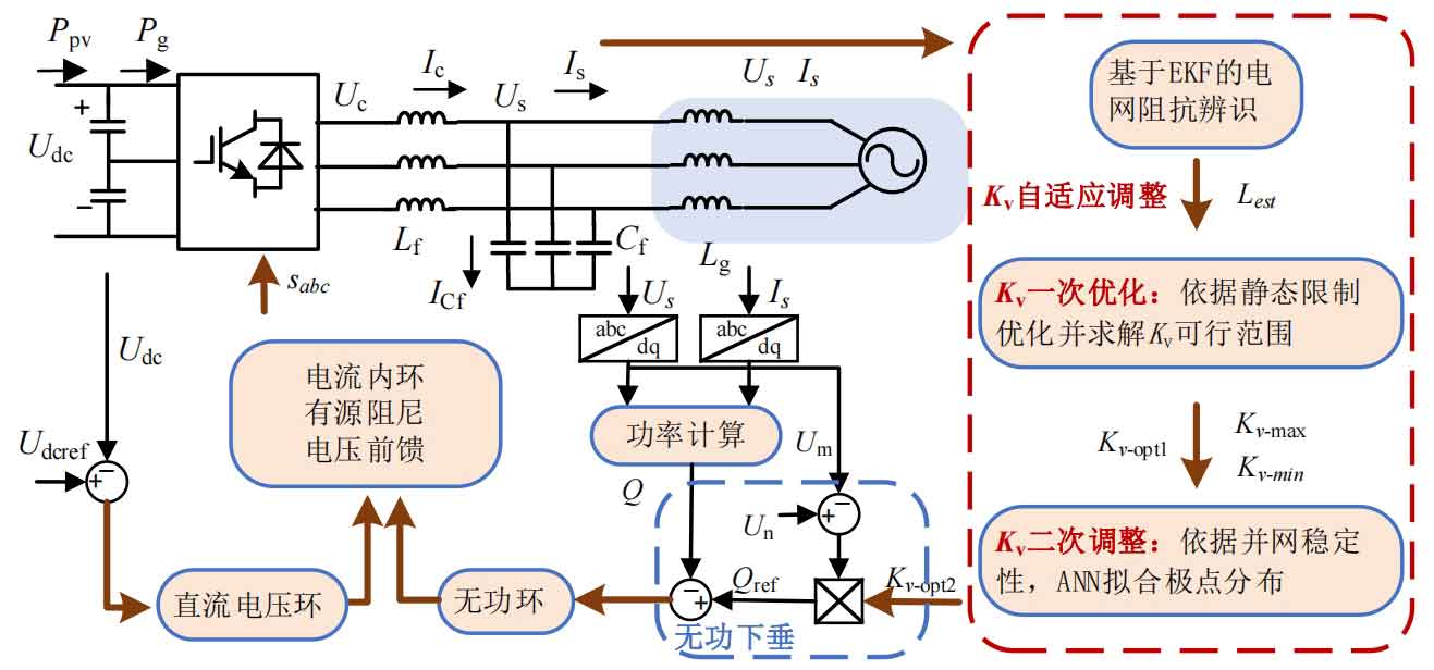
Figure 1 shows the overall control structure diagram of this article, where the red box represents the proposed control method. It can be seen that the method proposed in this article adds adaptive adjustment of the Q-V droop coefficient of the solar inverter on the basis of the conventional control structure. It mainly includes: optimizing the Q-V droop coefficient of the solar inverter once and solving the feasible range based on the output voltage and current limit, and judging the stability based on the ANN fitting system poles and adjusting the Q-V droop coefficient of the solar inverter twice. Finally, based on the impedance identification results of the power grid, the primary and secondary adaptive online adjustment of the Q-V droop coefficient of the solar inverter is achieved. Figure 1 also shows the typical photovoltaic grid connected converter circuit structure considered in this article, mainly including voltage source converters, LC filters, and non ideal power grids. In the figure, Us and Uc represent the voltage at the grid connection point and the output voltage of the converter, Is and Ic represent the output current and filtering inductor current, Udc represents the DC voltage, Pg and Ppv represent the output power on the grid side and the output power on the photovoltaic PV side, Lest represents the grid impedance identification result, Kv represents the Q-V droop coefficient of the solar inverter in the figure, Kv opt1 Kv opt2 represents the results of the first optimization and second adjustment of the Q-V droop coefficient of the solar inverter, where Um represents the voltage amplitude at the grid connection point and Un represents the set voltage reference.
2. Static feasible region analysis and work point optimization
This section analyzes voltage, current constraints, and active output to solve the Q-V droop coefficient of solar inverters, achieving a one-time optimization of the Q-V droop coefficient of solar inverters. Considering that the steady-state voltage and current output of the system and their phase relationship determine all operating states of the system (such as active and reactive power), this article refers to them as the “operating point” of the system.
For a photovoltaic converter, its output current is limited by the maximum current that the converter device can withstand, and the grid connection voltage is limited by the requirements of the power grid and the requirements for normal operation of the converter. This article limits the voltage Us within the range of 0.95-1.1 p.u. and Is below 1.2 p.u. The photovoltaic power generation side usually adopts MPPT control, with power as its control objective, while maintaining a constant DC voltage on the grid connected inverter side is the control objective. Therefore, in inverter control, the limiting conditions also include the output active power (determined by the MPPT control command of the photovoltaic PV side boost circuit).
After obtaining the limitations of the work point, the work point can be optimized. Due to the importance of voltage at the grid connection point for the normal operation of the system, the optimization objective for the operating point is to minimize the difference between the grid connection point voltage and the rated voltage. At the same time, the constraints on the working point are also reflected in the limitation on the maximum power value. The optimization problems for solving the working point and output power can be summarized as follows (the left optimization problem optimizes Kv, and the right optimization problem solves the maximum power Psmax):
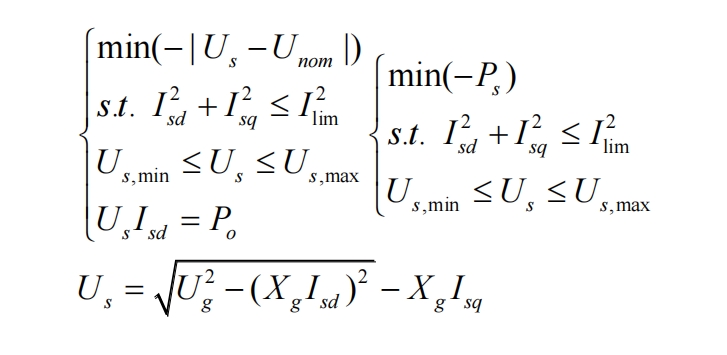
Among them, Us represents the grid voltage, Unom represents the rated voltage, Isd and Isq represent the components of the output current in the dq coordinate system, Po represents the photovoltaic power generation, Kv represents the Q-V droop coefficient of the solar inverter, and Xg represents the equivalent impedance of the grid. The result of optimizing the working point is the optimal working point of the system. Based on this working point, the corresponding Q-V droop coefficient of the solar inverter can be calculated. The calculation formula is as follows:
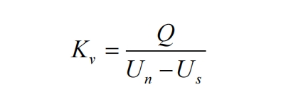
Among them, Un represents the droop control voltage reference setting value (in order to achieve a voltage of 1.1 p.u. at the grid connection point, the voltage reference setting value is set to 1.2 p.u.), and Q represents the reactive power output to the grid.
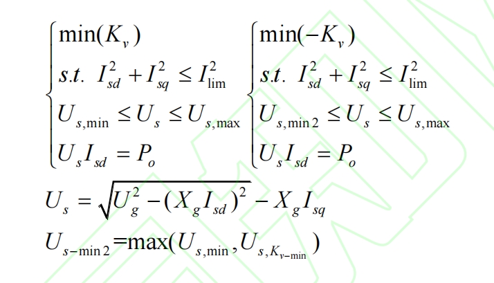
Under the condition of a certain output power, the maximum and minimum values of Kv under constraints can be obtained by solving the following optimization problems (the left optimization problem solves the minimum value of Kv, and the right optimization problem solves the maximum value of Kv).
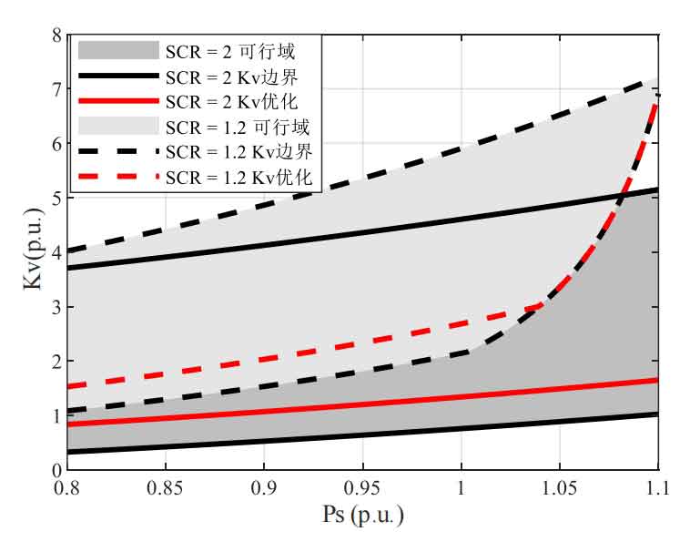
Draw the Kv optimization results and boundary solution results under different short circuit ratios (SCR) and output powers in different power grids, as shown in Figure 2. It can be seen that with the increase of SCR and Ps, the optimization results and feasible interval endpoint values of Kv increase, and when they increase to a certain extent, the optimization results of Kv coincide with the lower boundary of Kv. It is worth mentioning that the output power cannot be infinitely increased. When the output power is too large, any operating point will cause voltage or current to exceed the limit. In this case, it is necessary to issue a command to limit the active power output to the PV side boost circuit control.
3. One time optimization implementation method for Q-V droop coefficient of solar inverters
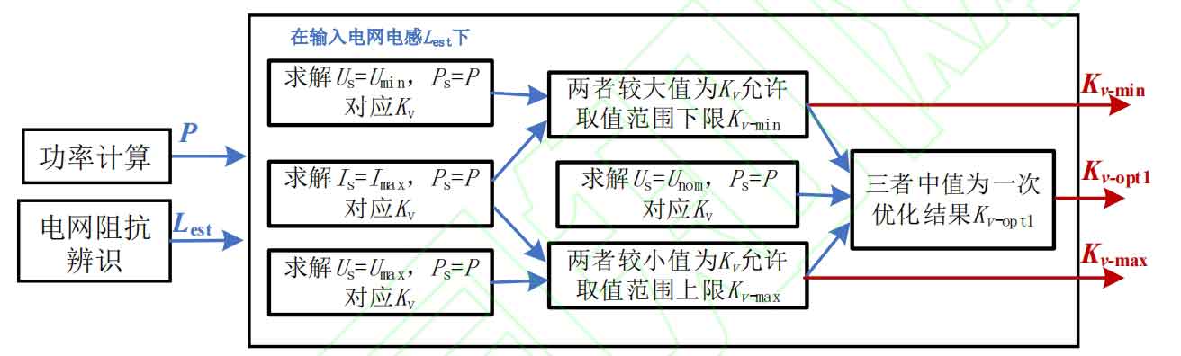
The solution process in the introduction of Kv’s one-time adjustment principle in the previous text is to solve multi constraint optimization problems. However, iterative solving of optimization problems usually requires a lot of computing resources, which is not conducive to online computing. Therefore, this article summarizes the optimization process into algorithmic solving to save computing resources. The schematic diagram of the algorithm is shown in Figure 3. The minimum value of Kv is solved by comparing the results of solving the minimum voltage limit and maximum current limit operating points Kv, the maximum value of Kv is solved by comparing the results of solving the maximum voltage limit and maximum current limit operating points Kv, and Kv opt1 is solved by comparing the results of solving the optimal voltage value operating point Kv with the minimum value of the maximum value.
Through the above process, the first optimization result and feasible range of the Q-V droop coefficient of the solar inverter that meets the active power output and the above electrical constraints can be obtained. However, to ensure the grid connection stability under this active power condition and the Q-V droop coefficient of the solar inverter, a second optimization adjustment considering stability constraints is needed, as follows.