
As a researcher in power electronics, I have long been fascinated by the intricate behaviors of utility interactive inverters, which serve as the critical interface between distributed energy resources and the utility grid. These systems are inherently nonlinear, and their stability is paramount for reliable operation. In this article, I will delve into the nonlinear dynamics of a specific utility interactive inverter based on the H6 topology under quasi-proportional-resonant (quasi-PR) control. The utility interactive inverter is a cornerstone of modern renewable energy systems, and understanding its complex behaviors is essential for robust design. I will explore the system’s discrete modeling, analyze its bifurcation and chaos phenomena, and demonstrate an effective control strategy to mitigate instability. Throughout, I will use mathematical formulations, tables, and analysis to provide a deep insight into the utility interactive inverter’s behavior, ensuring that the term ‘utility interactive inverter’ is prominently featured to emphasize its relevance.
The proliferation of photovoltaic (PV) systems has elevated the importance of utility interactive inverters, which must efficiently convert DC power to AC power while synchronizing with the grid. Nonlinearities in these utility interactive inverters can lead to undesirable dynamics such as bifurcations and chaos, potentially causing system failure. Traditional H-bridge utility interactive inverters face limitations like high leakage currents and efficiency issues. The H6 topology, with its additional diodes, offers improved performance by enabling three-level output and reducing common-mode voltages, making it a promising candidate for utility interactive inverter applications. However, the control strategy plays a pivotal role in stability. Quasi-PR control is advantageous for grid-tied systems due to its ability to suppress grid voltage disturbances and achieve zero steady-state error at the fundamental frequency. In this study, I focus on the nonlinear behavior of the utility interactive inverter with H6 structure under quasi-PR regulation, aiming to uncover the stability boundaries and control mechanisms.
To begin, let me outline the working principle of the utility interactive inverter. The H6 topology, as shown in the figure, consists of six switches (S1 to S6) and two diodes (D1 and D2). The utility interactive inverter connects to the grid through filter inductors L1 and L2, with parasitic resistances R1 and R2. The grid voltage is denoted as $u_g = U_m \sin(2\pi f t)$, and the reference current is $i_{ref} = I_m \sin(2\pi f t)$. The quasi-PR controller processes the error between $i_{ref}$ and the grid current $i_g$ to produce a control voltage $u_{con}$, which is compared with a triangular carrier wave to generate PWM signals for the switches. This utility interactive inverter operates in four modes during each output cycle, depending on the polarity of $i_g$ and the switching states. The key to analyzing nonlinearities is to derive a discrete-time model that captures the system’s dynamics at switching instants.
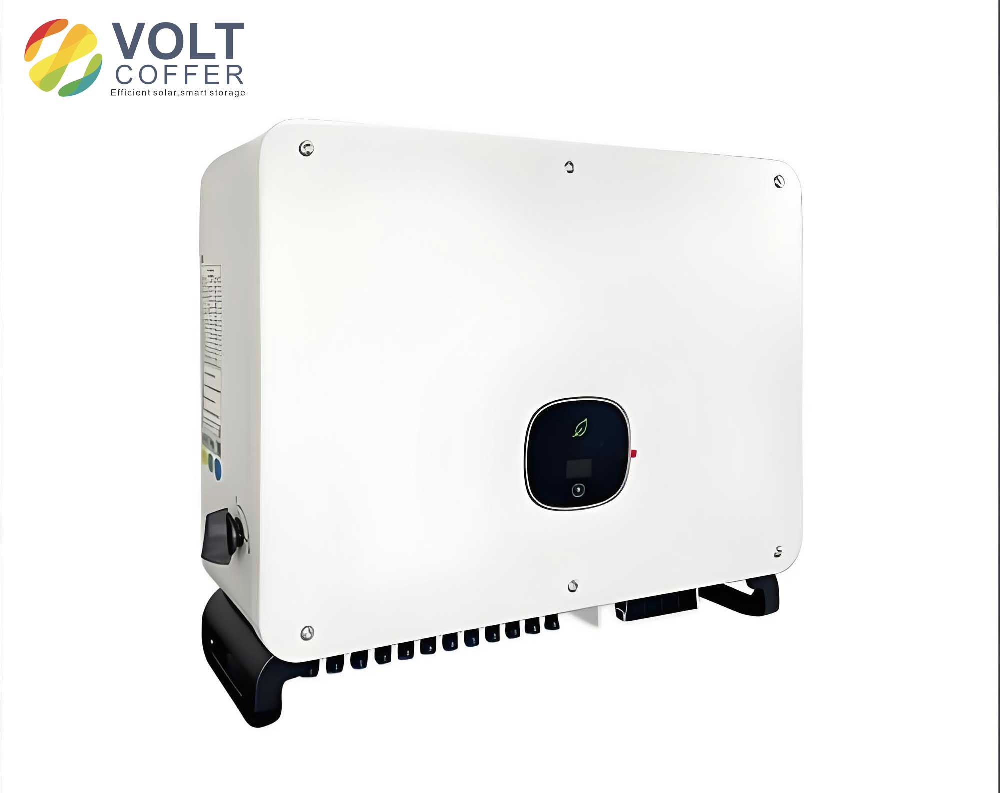
I employ the stroboscopic mapping method to develop a discrete iterative model for the utility interactive inverter. By sampling at the switching period $T$, I define $i_{g,n}$ as the grid current at time $nT$. The system’s state equations vary based on the sign of $i_g$. For $i_g > 0$, during the charging mode (modes 1 and 2), the dynamics are described by:
$$ \frac{di_g}{dt} = -\frac{R}{L} i_g + \frac{E}{2L} – \frac{u_g}{2L}, \quad \text{for } nT \leq t < (n+d_n)T $$
$$ \frac{di_g}{dt} = -\frac{R}{L} i_g – \frac{u_g}{2L}, \quad \text{for } (n+d_n)T \leq t \leq (n+1)T $$
where $d_n$ is the duty cycle in the $n$-th switching period, $E$ is the DC input voltage, $L = L_1 = L_2$, and $R = R_1 = R_2$. Discretizing these equations yields the iterative map for $i_g > 0$:
$$ i_{g,n+1} = e^{AT} i_{g,n} + e^{A(1-d_n)T} (e^{Ad_n T} – 1) A^{-1} B_1 E + [e^{A(1-d_n)T} – 1] A^{-1} B_2 E $$
with $A = -R/L$, $B_1 = 1/(2L) – u_{g,n}/(2LE)$, and $B_2 = -u_{g,n}/(2LE)$. Similarly, for $i_g < 0$, the utility interactive inverter operates in modes 3 and 4, leading to:
$$ i_{g,n+1} = e^{AT} i_{g,n} + e^{A(1-d_n)T} (e^{Ad_n T} – 1) A^{-1} B_3 E + [e^{A(1-d_n)T} – 1] A^{-1} B_4 E $$
where $B_3 = -1/(2L) – u_{g,n}/(2LE)$ and $B_4 = -u_{g,n}/(2LE)$. The quasi-PR controller adds complexity. Its transfer function is:
$$ G(s) = K_p + \frac{2K_r \omega_c s}{s^2 + 2\omega_c s + \omega_0^2} $$
where $K_p$ is the proportional gain, $K_r$ is the resonant gain, $\omega_c$ is the cutoff frequency, and $\omega_0 = 2\pi f$ is the resonant frequency. By defining state variables $Y = [y_1, y_2]^T$, I express the controller in state-space form and discretize it to obtain:
$$ Y_{n+1} = e^{G T} Y_n + (e^{G T} – I) G^{-1} F (i_{ref,n} – i_{g,n}) $$
$$ u_{con,n} = H Y_n + K_p (i_{ref,n} – i_{g,n}) $$
with $G = \begin{bmatrix} 0 & 1 \\ -\omega_0^2 & -2\omega_c \end{bmatrix}$, $F = [0, 1]^T$, and $H = [0, 2K_r \omega_c]$. The duty cycle $d_n$ is then derived from PWM comparison:
$$ d_n = H Y_n + K_p (i_{ref,n} – i_{g,n}) \quad \text{for } i_{ref,n} \geq 0 $$
$$ d_n = -H Y_n – K_p (i_{ref,n} – i_{g,n}) \quad \text{for } i_{ref,n} < 0 $$
with saturation limits $0 \leq d_n \leq 1$. The complete discrete model of the utility interactive inverter consists of these equations, enabling numerical analysis of nonlinear dynamics. This model is crucial for studying the utility interactive inverter’s behavior under varying parameters.
Next, I analyze the nonlinear behavior of the utility interactive inverter using bifurcation diagrams, folding diagrams, Lyapunov exponents, and time-domain simulations. The primary parameter of interest is the proportional gain $K_p$, as it directly influences stability. For default parameters (e.g., $E = 450\,V$, $L = 8.5\,mH$, $f_s = 5\,kHz$, $K_r = 100$), I vary $K_p$ from 0 to 1 and observe the grid current $i_g$ at peak instances. The bifurcation diagram reveals rich dynamics: for $0 < K_p \leq 0.11$, the utility interactive inverter exhibits Hopf bifurcation leading to low-frequency oscillations; for $0.11 < K_p \leq 0.42$, it operates stably in period-1; and for $0.42 < K_p \leq 0.6$, period-doubling bifurcation occurs, followed by border collision bifurcation into chaos. This is confirmed by the maximum Lyapunov exponent, which turns positive in chaotic regions. To illustrate, I summarize the stability regions for $K_p$ in a table:
| Parameter Range | System Behavior | Stability Status |
|---|---|---|
| $0 < K_p \leq 0.11$ | Hopf bifurcation, low-frequency oscillations | Unstable |
| $0.11 < K_p \leq 0.42$ | Period-1 operation | Stable |
| $0.42 < K_p \leq 0.6$ | Period-doubling and border collision bifurcation to chaos | Unstable |
The folding diagrams for specific $K_p$ values, such as $K_p = 0.105$ (oscillatory), $K_p = 0.3$ (stable), and $K_p = 0.5$ (chaotic), visually corroborate these states. Time-domain waveforms and their Fast Fourier Transform (FFT) spectra further validate the analysis: in chaotic mode, the utility interactive inverter shows aperiodic waveforms with high total harmonic distortion (THD), whereas stable operation yields clean sinusoidal currents. This underscores the sensitivity of the utility interactive inverter to control parameters.
Beyond $K_p$, other parameters significantly affect the utility interactive inverter’s stability. I explore the resonant gain $K_r$, input voltage $E$, and filter inductance $L$ through bifurcation analysis. For $K_r$, as it increases from 0 to 500, the utility interactive inverter remains stable until $K_r \approx 244$, after which Hopf bifurcation induces chaos. For $E$, stability holds for $400\,V \leq E < 705\,V$, with period-doubling bifurcation beyond that. For $L$, stability requires $L \geq 5.5\,mH$, and reducing $L$ leads to period-doubling bifurcation. These findings highlight the interdependencies in the utility interactive inverter design. I consolidate the stable operating ranges in a table:
| Parameter | Stable Range | Bifurcation Type Beyond Range |
|---|---|---|
| $K_r$ | $0 \leq K_r < 244$ | Hopf bifurcation to chaos |
| $E$ | $400\,V \leq E < 705\,V$ | Period-doubling bifurcation to chaos |
| $L$ | $L \geq 5.5\,mH$ | Period-doubling bifurcation to chaos |
Moreover, I investigate two-dimensional stability boundaries to understand parameter interactions. For instance, in the $K_p$-$K_r$ plane, the stable region is centrally located, bounded by unstable zones above and below. Similarly, in the $E$-$L$ plane, stability dominates at lower $E$ and higher $L$, with instability creeping in as $E$ increases or $L$ decreases. These boundaries are essential for designing a robust utility interactive inverter, as they define safe operational envelopes. The utility interactive inverter’s performance is thus a delicate balance of multiple factors, necessitating comprehensive nonlinear analysis.
To address instability, I propose a chaos control method using a second-order band-reject filter. When the utility interactive inverter enters chaotic states (e.g., at $K_p = 0.5$), introducing this filter can suppress unwanted oscillations. The filter’s transfer function is:
$$ F(s) = K_z \frac{s^2 + \omega_b^2}{s^2 + 2\omega_b s + \omega_b^2} $$
where $K_z = 0.1$ is the control coefficient and $\omega_b = 314\,rad/s$ is the center frequency. By integrating $F(s)$ into the control loop, it extracts non-fundamental components from $i_g$ and feeds them back to the controller, effectively damping chaos. Discretizing the filter yields additional state equations that modify the control voltage $u_{con,n}$. Applying this control to the utility interactive inverter demonstrates remarkable recovery: time-domain waveforms show that chaotic or period-doubled states revert to stable period-1 operation. For example, at $E = 800\,V$ (chaotic without control), the utility interactive inverter stabilizes post-control; similarly, at $L = 5.3\,mH$ (period-doubling), control restores stability. This underscores the efficacy of the band-reject filter in enhancing the utility interactive inverter’s resilience.
I further analyze the impact of control on parameter stability domains. With the band-reject filter, the stable range for $K_p$ shifts slightly to $0.22 < K_p \leq 0.53$, while $K_r$’s stable range reduces to $0 \leq K_r < 164$ due to the filter’s attenuation at resonant frequency. However, the utility interactive inverter benefits significantly in terms of $E$ and $L$: the stable input voltage expands to $400\,V \leq E < 1312\,V$, and the stable inductance extends to $L \geq 3\,mH$. These expansions are crucial for practical utility interactive inverter applications, where input variations and component tolerances are common. I summarize the controlled stability ranges below:
| Parameter | Stable Range Without Control | Stable Range With Control | Improvement |
|---|---|---|---|
| $K_p$ | $0.11 < K_p \leq 0.42$ | $0.22 < K_p \leq 0.53$ | Shifted, similar width |
| $K_r$ | $0 \leq K_r < 244$ | $0 \leq K_r < 164$ | Reduced due to filter |
| $E$ | $400\,V \leq E < 705\,V$ | $400\,V \leq E < 1312\,V$ | Significantly expanded |
| $L$ | $L \geq 5.5\,mH$ | $L \geq 3\,mH$ | Significantly expanded |
The band-reject filter thus not only controls chaos but also broadens the operational flexibility of the utility interactive inverter, making it more adaptable to real-world conditions. This is a key advantage for utility interactive inverters in renewable energy systems, where grid and load variations are frequent.
To validate these theoretical and numerical findings, I conduct experimental verification using a dSPACE-based hardware-in-the-loop platform. The utility interactive inverter is implemented with the same parameters as in simulations. For instance, at $K_p = 0.5$, the uncontrolled utility interactive inverter exhibits chaotic current ripple with amplitudes up to 3A and no fixed period; after applying the band-reject filter control, the ripple reduces to 1A with a regular switching period. Similarly, at $E = 800\,V$, control tames the chaos, and at $L = 5.3\,mH$, it eliminates period-doubling. These experimental results align perfectly with simulations, confirming the discrete model’s accuracy and the control strategy’s effectiveness. The utility interactive inverter’s behavior under various conditions thus serves as a testament to the importance of nonlinear analysis in power electronics design.
In conclusion, the utility interactive inverter with H6 topology and quasi-PR control exhibits complex nonlinear dynamics, including Hopf bifurcation, period-doubling bifurcation, and border collision bifurcation leading to chaos. Through discrete modeling and numerical tools, I have mapped the stability boundaries for key parameters like $K_p$, $K_r$, $E$, and $L$. The introduction of a second-order band-reject filter proves to be an effective chaos control method, not only stabilizing the utility interactive inverter but also expanding the stable operating ranges for input voltage and filter inductance. This study provides valuable insights for engineers designing utility interactive inverters, emphasizing the need to consider nonlinear behaviors during parameter tuning. Future work could explore adaptive control schemes or other filter designs to further enhance the utility interactive inverter’s performance. Ultimately, a deep understanding of these dynamics ensures that utility interactive inverters can operate reliably in diverse grid conditions, supporting the global transition to sustainable energy.
Throughout this analysis, the term ‘utility interactive inverter’ has been central, highlighting its role in modern power systems. The H6-based utility interactive inverter, with its improved efficiency and reduced leakage current, represents a significant advancement, but its control must be carefully crafted to avoid instability. By leveraging nonlinear dynamics principles, we can unlock the full potential of utility interactive inverters, making them more robust and efficient. I hope this comprehensive exploration serves as a resource for researchers and practitioners alike, fostering innovation in utility interactive inverter technology.