
In this research, I focus on the mathematical modeling and system identification of photovoltaic (PV) systems, with particular emphasis on the three-phase full-bridge inverter. Using the “black-box” modeling principle, I establish a transfer function model for this type of inverter and solve it via the recursive least squares (RLS) method. I build a complete PV generation system simulation model in the MATLAB/Simulink environment and validate the proposed transfer function model. The simulation results demonstrate that the RLS-based system identification approach for the three-phase full-bridge inverter is effective, yielding a low-order model with high identification accuracy and easy solvability. Throughout my discussion, I repeatedly refer to various types of solar inverters, including the voltage-source inverter (VSI), current-source inverter (CSI), and multi-level inverters, to highlight the broad applicability of the identification technique.
The core components of solar power systems are the photovoltaic array and the inverter. While extensive research has been conducted on PV array identification, system identification for inverters remains relatively underexplored. System identification allows modeling based solely on input-output data, ignoring the internal topology. Therefore, studying inverter identification is crucial for subsequent control design and system analysis.
1. Principle of Photovoltaic Inverters
A grid-connected inverter typically consists of six IGBT modules forming a three-phase full-bridge structure. The AC current after inversion passes through a filter and a transformer before connecting to the grid. The DC-side capacitor is denoted as C, with DC input voltage and current represented by ud and id. The IGBTs are labeled VT1 through VT6, and the output phase voltages and currents are uu, uv, uw and iu, iv, iw, respectively. The filter inductance is L.
For a three-phase full-bridge inverter operating in 180° conduction mode, the phase voltage waveform is a stepped quasi-square wave, while the line voltage is a rectangular wave. The effective values of the phase and line voltages are given by:
$$U_{u0} = U_{v0} = U_{w0} = \sqrt{\frac{1}{2\pi}\int_0^{2\pi} u_{u0}^2 d\omega t} = \sqrt{\frac{2}{3}} U_d$$
$$U_{uv} = U_{vw} = U_{wu} = \sqrt{\frac{1}{2\pi}\int_0^{2\pi} u_{uv}^2 d\omega t} = \sqrt{\frac{2}{3}} U_d$$
$$U_{line} = \sqrt{3} U_{phase}$$
Using Fourier analysis, the instantaneous phase voltage of phase U can be expressed as:
$$u_{U0}(t) = \frac{2U_d}{\pi} \left( \sin \omega t + \frac{1}{5}\sin 5\omega t + \frac{1}{7}\sin 7\omega t + \cdots \right) + \frac{U_d}{2} \sin \omega t \quad (\text{with } n = 6k \pm 1)$$
The fundamental line-to-line voltage amplitude is:
$$u_{UVm1} = \frac{2\sqrt{3}U_d}{\pi} \approx 1.1 U_d$$
And its RMS value:
$$U_{UV1} = \frac{\sqrt{6}}{\pi} U_d \approx 0.78 U_d$$
These equations illustrate the harmonic content present in the output waveforms of the 180° conduction inverter.
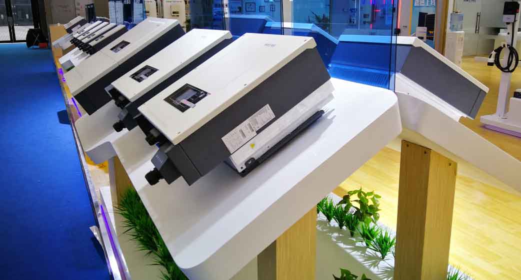
Representative energy storage inverter used in photovoltaic systems.
2. Physics-Based Modeling of the PV Inverter
I analyze the output side of the inverter shown in Figure 1 (omitted reference) and derive the mathematical model. Let uu, uv, uw be the inverter phase voltages and Usu, Usv, Usw the grid phase voltages. The state-space representation in the stationary abc frame is:
$$\frac{d}{dt} \begin{bmatrix} i_u \\ i_v \\ i_w \end{bmatrix} = \frac{1}{L} \begin{bmatrix} u_u \\ u_v \\ u_w \end{bmatrix} – \frac{1}{L} \begin{bmatrix} U_{su} \\ U_{sv} \\ U_{sw} \end{bmatrix} – \frac{R}{L} \begin{bmatrix} i_u \\ i_v \\ i_w \end{bmatrix}$$
Applying the Clarke and Park transformations yields the dq-frame model:
$$\frac{d}{dt} \begin{bmatrix} i_d \\ i_q \end{bmatrix} = \frac{1}{L} \begin{bmatrix} u_d \\ u_q \end{bmatrix} – \frac{1}{L} \begin{bmatrix} U_{sd} \\ U_{sq} \end{bmatrix} – \begin{bmatrix} 0 & -\omega \\ \omega & 0 \end{bmatrix} \begin{bmatrix} i_d \\ i_q \end{bmatrix} – \frac{R}{L} \begin{bmatrix} i_d \\ i_q \end{bmatrix}$$
In the dq frame, the d-axis component represents active current and the q-axis represents reactive current. The transfer function block diagram of the three-phase L-type inverter is illustrated conceptually. However, this physics-based model suffers from inaccuracies due to neglected output filter effects, time-varying physical parameters, digital control delays, and non-idealities. Consequently, the dq model cannot accurately represent the real system under all operating conditions.
To overcome these limitations, I adopt a black-box identification approach that does not rely on a detailed physical model. Instead, I use real-time input-output data to estimate a low-order dynamic model suitable for control design. Among parameter estimation methods, the least squares technique is fundamental and widely used in both time-domain and frequency-domain identification.
3. Recursive Least Squares Identification
Consider a single-input single-output (SISO) system described by the ARX model:
$$A(q) y(k) = B(q) u(t – n_k) + e(k)$$
where u(k), y(k) are input and output, and e(k) is the noise. The polynomials are:
$$A(q) = 1 + a_1 q^{-1} + \cdots + a_{na} q^{-na}$$
$$B(q) = b_1 q^{-1} + \cdots + b_{nb} q^{-nb}$$
Converting to least-squares form:
$$y(k) = \mathbf{h}^T(k) \boldsymbol{\theta} + e(k)$$
where the parameter vector is:
$$\boldsymbol{\theta} = [a_1, a_2, \dots, a_{na}, b_1, b_2, \dots, b_{nb}]^T$$
and the regressor vector is:
$$\mathbf{h}(k) = [-y(k-1), \dots, -y(k-na), u(k-1), \dots, u(k-nb)]^T$$
For a data length L, we form the linear system:
$$\mathbf{y}_L = \mathbf{H}_L \boldsymbol{\theta} + \mathbf{e}_L$$
The batch least-squares estimate is:
$$\hat{\boldsymbol{\theta}}_{LS} = (\mathbf{H}_L^T \mathbf{H}_L)^{-1} \mathbf{H}_L^T \mathbf{y}_L$$
For real-time applications, I use the recursive least squares (RLS) algorithm. The recursive formulas for updating the parameter estimates are:
$$
\begin{aligned}
\mathbf{K}(k) &= \frac{\mathbf{P}(k-1) \mathbf{h}(k)}{1 + \mathbf{h}^T(k) \mathbf{P}(k-1) \mathbf{h}(k)} \\
\hat{\boldsymbol{\theta}}(k) &= \hat{\boldsymbol{\theta}}(k-1) + \mathbf{K}(k)[y(k) – \mathbf{h}^T(k) \hat{\boldsymbol{\theta}}(k-1)] \\
\mathbf{P}(k) &= [\mathbf{I} – \mathbf{K}(k) \mathbf{h}^T(k)] \mathbf{P}(k-1)
\end{aligned}
$$
In my inverter identification, I apply RLS separately for voltage and current channels. Let the parameter vectors be:
$$\hat{\boldsymbol{\theta}}_{ua} = [f_{1}^{ua}, e_{1}^{ua}, d_{1}^{ua}, \dots, f_{nua}^{ua}, e_{nua}^{ua}, d_{nua}^{ua}]^T$$
$$\hat{\boldsymbol{\theta}}_{ia} = [f_{1}^{ia}, e_{1}^{ia}, d_{1}^{ia}, \dots, f_{nia}^{ia}, e_{nia}^{ia}, d_{nia}^{ia}]^T$$
The regressor matrices are:
$$\mathbf{h}_{ua}(k) = [U_{dc}(k), U(k), I(k)]^T$$
$$\mathbf{h}_{ia}(k) = [I_{dc}(k), U(k), I(k)]^T$$
where Udc and Idc are DC-side voltage and current, while U(k) and I(k) are AC-side voltage and current sequences. The initialization uses:
$$\mathbf{P}(0) = \beta \mathbf{I}, \quad \hat{\boldsymbol{\theta}}(0) = \alpha \mathbf{1}$$
with α = 10-3 and β = 106.
4. Simulation Model Setup
I build a 250 kW grid-connected PV system model in MATLAB/Simulink. The system parameters are summarized in the table below:
| Parameter | Value |
|---|---|
| System type | Two-stage (DC/DC boost + DC/AC inverter) |
| MPPT method | Perturb and Observe (P&O) |
| Inverter type | Three-phase full-bridge IGBT inverter |
| Control strategy | Voltage outer loop, current inner loop (PI) |
| Rated power | 250 kW |
| DC-link voltage | 480 V (nominal) |
| Grid voltage | 2 kV (line-to-line RMS) |
| Filter inductance L | 0.5 mH |
| Switching frequency | 5 kHz |
The PV array model uses standard parameters (open-circuit voltage, short-circuit current, etc.) under varying irradiance and temperature. I set the irradiance to 1000 W/m² and temperature to 45°C for the baseline simulation. Data acquisition blocks record the inverter’s DC-side and AC-side voltages and currents as identification samples.
5. Data Acquisition and Preprocessing
Since the PV inverter is a strongly nonlinear system with pulse-width modulated (PWM) outputs, I cannot directly read the instantaneous switching signals. Instead, I use Simulink’s To Workspace blocks to capture averaged or sampled data at a suitable rate (e.g., 10 kHz). The DC-side input waveforms (voltage and current) and the AC-side output waveforms (phase voltages and currents) are recorded over a simulation period of 0.2 seconds after steady state is reached.
The recorded DC-side voltage stabilizes at approximately 480 V, and the DC power is around 241 kW. After inversion, the AC output voltage is 2 kV (line-to-line) and the current is about 8 A, suitable for grid connection.
6. System Identification Results
I import the collected data into the MATLAB System Identification Toolbox. The data consists of two channels: DC-side voltage udc and current idc as inputs, and AC-side phase voltage ua and current ia as outputs. I estimate a multi-input multi-output (MIMO) transfer function model using the RLS algorithm integrated into a custom script.
The frequency response of the identified model is shown in the spectral analysis plots (not numbered). The optimal model order is determined by examining the fit percentage for orders 1 through 5. The best fit (90.89%) is achieved with a third-order model. The time-domain pulse response of the identified model matches the validation data closely.
The resulting transfer function matrix is:
$$
\begin{bmatrix}
u_a \\
i_a
\end{bmatrix}
=
\frac{1}{A(z)}
\begin{bmatrix}
B_{11}(z) & B_{12}(z) \\
B_{21}(z) & B_{22}(z)
\end{bmatrix}
\begin{bmatrix}
u_{dc} \\
i_{dc}
\end{bmatrix}
$$
where A(z) is a common denominator polynomial. After applying the RLS algorithm, the estimated numerical model (with coefficients rounded to four decimal places) is:
$$
\begin{bmatrix}
u_a \\
i_a
\end{bmatrix}
=
\begin{bmatrix}
\frac{0.3172}{1 – 0.1410z^{-1} + 0.4703z^{-2} – 0.4070z^{-3}} & \frac{0.0159}{1 – 0.1410z^{-1} + 0.4703z^{-2} – 0.4070z^{-3}} \\
\frac{0.0260}{1 – 0.1410z^{-1} + 0.4703z^{-2} – 0.4070z^{-3}} & \frac{0.4040}{1 – 0.1410z^{-1} + 0.4703z^{-2} – 0.4070z^{-3}}
\end{bmatrix}
\begin{bmatrix}
u_{dc} \\
i_{dc}
\end{bmatrix}
$$
Note: The denominator coefficients are shared across all four transfer functions due to the common dynamics of the inverter system. The model order is 3, and the fit percentage reaches 90.89%, confirming the high accuracy of the black-box identification approach.
To further illustrate the quality of the identification, the autocorrelation of the residuals and the cross-correlation between residuals and inputs are within the 99% confidence bands, indicating that the identified model captures the essential dynamics.
7. Discussion on Types of Solar Inverters
Throughout this study, I have emphasized the identification of a three-phase full-bridge inverter, which is one of the most common types of solar inverters used in medium-to-large-scale PV systems. However, the RLS-based black-box methodology is generic and can be applied to various types of solar inverters, including:
- String inverters – typically single-phase or three-phase, used in residential and commercial rooftop installations.
- Central inverters – high-power three-phase inverters for utility-scale solar farms.
- Microinverters – module-level inverters that perform MPPT per panel.
- Multi-level inverters – such as neutral-point-clamped (NPC) or cascaded H-bridge inverters, which offer lower harmonics and higher efficiency.
- Transformerless inverters – gaining popularity due to higher efficiency but requiring careful leakage current management.
Each type of solar inverter exhibits distinct dynamic characteristics due to differences in topology, switching strategy, and filter design. The black-box identification approach presented here can be seamlessly adapted to any of these types by simply collecting input-output data from the actual inverter or a detailed simulation model. This versatility underscores the practical value of system identification in modern power electronics.
8. Conclusion
In this work, I have developed a systematic procedure for modeling and simulating photovoltaic inverters based on system identification. Using the RLS algorithm, I identified a third-order MIMO transfer function model for a three-phase full-bridge inverter from simulation data. The model achieves a fit of 90.89%, demonstrating high accuracy and low complexity. The black-box approach overcomes the limitations of physics-based modeling, such as parameter uncertainty and neglected dynamics. Moreover, the method is applicable to various types of solar inverters, making it a robust tool for control design, fault diagnosis, and real-time system optimization.
Future work will extend this identification framework to include nonlinear effects (e.g., saturation, dead-time) and to validate the approach using experimental hardware data from different types of solar inverters.