
With the rapid development of new energy technologies, lithium-ion batteries have become indispensable in various fields such as consumer electronics, aerospace, and electric vehicles due to their high energy density, long lifespan, compact size, and low environmental impact. However, the capacity of lithium-ion batteries gradually degrades over repeated charge and discharge cycles, eventually leading to end-of-life and posing significant safety risks. Therefore, accurately predicting the State of Health (SOH) and Remaining Useful Life (RUL) of lithium-ion batteries is crucial for ensuring safety and optimizing system performance. Traditional prediction methods often require extensive historical data, which is challenging to obtain in practical applications where only limited degradation data is available. This paper addresses this issue by proposing a novel framework for joint SOH and RUL prediction under limited data conditions, leveraging multi-scale decomposition, dimensionality reduction, and a hybrid deep learning model.
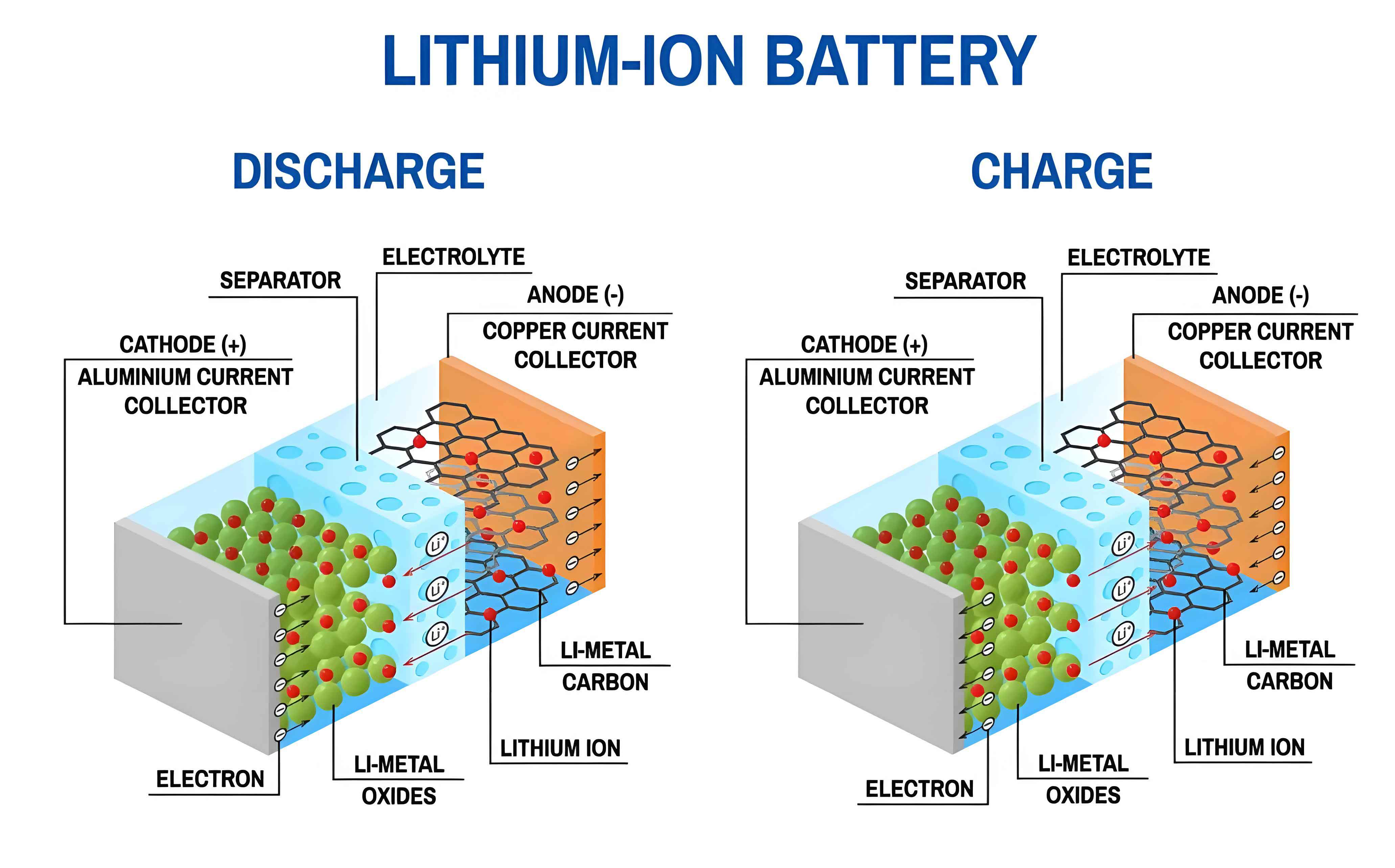
Existing approaches for degradation trajectory prediction can be broadly categorized into model-based and data-driven methods. Model-based methods, such as electrochemical models and equivalent circuit models, rely on precise physical representations but are often complex and computationally intensive. In contrast, data-driven methods, which include various machine learning and deep learning techniques, do not require explicit physical models and instead learn patterns from measured data. However, these methods typically demand large datasets for training, making them less suitable for scenarios with limited data. Recent studies have explored early prediction using only initial cycles of data, but challenges remain in handling noise, data quality, and feature extraction. This paper introduces a comprehensive framework that combines Complete Ensemble Empirical Mode Decomposition with Adaptive Noise (CEEMDAN), Principal Component Analysis (PCA), Convolutional Neural Networks (CNN), and Relevance Vector Machine (RVM) to achieve accurate SOH and RUL prediction with only the first 10% of capacity data.
Methodology
The proposed framework consists of three main stages: data preprocessing via CEEMDAN and PCA, feature extraction using CNN, and joint prediction via RVM. The overall flowchart is illustrated in Figure 1, but here we describe the mathematical foundations and implementation details.
Data Preprocessing with CEEMDAN and PCA
Given the limited data scenario, we extract the first 10% of the capacity degradation sequence from the lithium-ion battery. Let the original capacity signal be denoted as \( x(t) \), where \( t \) represents the cycle index. To handle non-stationary and nonlinear characteristics, we apply CEEMDAN, which adaptively decomposes \( x(t) \) into a set of Intrinsic Mode Functions (IMFs) and a residual. The CEEMDAN process involves adding Gaussian white noise to the signal and performing Empirical Mode Decomposition (EMD) iteratively. The steps are as follows:
1. Define the original signal \( x(t) \). Add Gaussian white noise \( G_i(t) \) to construct noisy signals: \( x_i(t) = x(t) + G_i(t) \), for \( i = 1, 2, \dots, n \), where \( n \) is the number of noise realizations.
2. Perform EMD on each \( x_i(t) \) to obtain the first IMF and residual. The first IMF component is computed as:
$$ I_{\text{IMF1}} = \frac{1}{n} \sum_{i=1}^{n} I_{\text{IMF1}}^i(t) $$
where \( I_{\text{IMF1}}^i(t) \) is the first IMF from the \( i \)-th decomposition. The residual is:
$$ r_1(t) = x(t) – I_{\text{IMF1}} $$
3. For the \( k \)-th stage (\( k \geq 2 \)), add noise to the residual \( r_{k-1}(t) \) and decompose to obtain the \( k \)-th IMF:
$$ I_{\text{IMF}k} = \frac{1}{n} \sum_{i=1}^{n} \text{EMD}(r_{k-1}(t) + \epsilon_{k-1} G_i(t)) $$
where \( \epsilon_{k-1} \) is an adaptive noise coefficient. The residual is updated as \( r_k(t) = r_{k-1}(t) – I_{\text{IMF}k} \).
4. Repeat until the residual contains no more than two extrema. The original signal can be reconstructed as:
$$ x(t) = \sum_{j=1}^{z} I_{\text{IMF}j} + r_z(t) $$
where \( z \) is the number of IMFs and \( r_z(t) \) is the final residual. This decomposition yields multiple IMFs representing different frequency components and a trend residual, which helps isolate noise and capture degradation patterns.
However, the high-dimensional IMFs may contain redundant or noisy information. To address this, we apply PCA for dimensionality reduction and feature fusion. Let the decomposed components be arranged into a data matrix \( \mathbf{X} \in \mathbb{R}^{m \times n} \), where \( m \) is the number of cycles and \( n \) is the number of components (IMFs plus residual). After standardizing \( \mathbf{X} \), we compute the covariance matrix \( \mathbf{C} \):
$$ \mathbf{C} = \frac{1}{m-1} \mathbf{X}^T \mathbf{X} $$
The eigenvalues \( \lambda_i \) and eigenvectors \( \mathbf{e}_i \) of \( \mathbf{C} \) are obtained by solving:
$$ \mathbf{C} \mathbf{e}_i = \lambda_i \mathbf{e}_i $$
The eigenvectors are sorted in descending order of eigenvalues, and the principal components (PCs) are formed by projecting the data onto these eigenvectors. The transformed data \( \mathbf{Z} \) is given by:
$$ \mathbf{Z} = \mathbf{X} \mathbf{V} $$
where \( \mathbf{V} \) is the matrix of selected eigenvectors. We retain PCs that cumulatively explain over 99% of the variance, effectively reducing dimensionality while preserving essential degradation information. This step enhances data quality and mitigates noise interference.
Feature Extraction with Convolutional Neural Network (CNN)
The reduced-dimensional data from PCA is then fed into a CNN to extract deep features that capture local correlations and degradation trends. A CNN typically consists of convolutional layers, activation functions, pooling layers, and fully connected layers. For a given input feature map \( \mathbf{X} \), the convolution operation at layer \( l \) is defined as:
$$ \mathbf{O}^l = f\left( \sum_{i=1}^{N} \mathbf{X} \ast \mathbf{K}_i^l + \mathbf{b}_i^l \right) $$
where \( \ast \) denotes convolution, \( \mathbf{K}_i^l \) is the \( i \)-th kernel in layer \( l \), \( \mathbf{b}_i^l \) is the bias, \( N \) is the number of kernels, and \( f(\cdot) \) is the activation function (ReLU is used here). The pooling layer downsamples the feature maps to reduce computational cost and prevent overfitting. Max pooling is applied as:
$$ \mathbf{O}^l(j) = \max_{t \in \text{window}} \mathbf{X}^{l-1}(t) $$
where \( \mathbf{O}^l(j) \) is the output at position \( j \), and the window defines the local region. The CNN architecture in this work includes multiple convolutional and pooling layers, followed by flattening and fully connected layers to produce high-level features for subsequent prediction.
Joint Prediction with Relevance Vector Machine (RVM)
The features extracted by CNN are used as inputs to an RVM model for joint SOH and RUL prediction. RVM is a Bayesian sparse kernel model that offers probabilistic outputs and requires fewer support vectors compared to Support Vector Machines (SVM). Given a training dataset \( \{ \mathbf{x}_i, t_i \}_{i=1}^{N} \), where \( \mathbf{x}_i \) is the feature vector and \( t_i \) is the target value (SOH or RUL), the RVM model assumes:
$$ t_i = y(\mathbf{x}_i) + \epsilon_i $$
with \( \epsilon_i \sim \mathcal{N}(0, \sigma^2) \). The function \( y(\mathbf{x}) \) is expressed as:
$$ y(\mathbf{x}) = \sum_{i=1}^{N} \omega_i K(\mathbf{x}, \mathbf{x}_i) + \omega_0 $$
where \( \omega_i \) are weights, \( K(\cdot, \cdot) \) is a kernel function (e.g., radial basis function), and \( \omega_0 \) is the bias. In matrix form, \( \mathbf{t} = \mathbf{\Phi} \mathbf{\omega} + \mathbf{\epsilon} \), where \( \mathbf{\Phi} \) is the design matrix with elements \( \Phi_{ij} = K(\mathbf{x}_i, \mathbf{x}_j) \).
RVM imposes a Gaussian prior on the weights to promote sparsity:
$$ p(\mathbf{\omega} | \mathbf{\alpha}) = \prod_{i=0}^{N} \mathcal{N}(\omega_i | 0, \alpha_i^{-1}) $$
where \( \mathbf{\alpha} \) is a vector of hyperparameters. The posterior distribution of weights is computed using Bayesian inference, and the hyperparameters are optimized via evidence maximization. This results in a sparse model where many weights are zero, making predictions efficient and interpretable. For joint prediction, we train separate RVM models for SOH and RUL, but they share the same CNN-extracted features, enabling a unified framework.
Experimental Setup and Evaluation Metrics
To validate the proposed framework, we use publicly available lithium-ion battery datasets from the University of Maryland’s Center for Advanced Life Cycle Engineering (CALCE) and Tongji University (TJU). These datasets include batteries with different chemistries, capacities, and operating conditions, as summarized in Table 1.
| Battery | Protocol | Ambient Temperature (°C) | Charge Cut-off Voltage (V) | Discharge Cut-off Voltage (V) | Capacity (Ah) | Total Cycles |
|---|---|---|---|---|---|---|
| CS2-35 | CC-CV | 24 | 4.2 | 2.7 | 1.1 | 717 |
| CS2-36 | CC-CV | 24 | 4.2 | 2.7 | 1.1 | 694 |
| CY25-025/1-#1 | CC-CV | 25 | 4.2 | 2.65 | 3.5 | 488 |
| CY35-05/1-#1 | CC-CV | 35 | 4.2 | 2.65 | 3.5 | 570 |
The SOH is defined as the ratio of current maximum available capacity to nominal capacity:
$$ \text{SOH} = \frac{Q_{\text{current}}}{Q_{\text{nominal}}} \times 100\% $$
RUL is defined as the number of remaining cycles until the capacity drops to 80% of the nominal capacity (end-of-life threshold). For evaluation, we use the following metrics: Mean Absolute Percentage Error (MAPE), Mean Absolute Error (MAE), Root Mean Square Error (RMSE), and RUL error in cycles.
$$ \text{MAPE} = \frac{1}{N} \sum_{i=1}^{N} \left| \frac{y_i – \hat{y}_i}{y_i} \right| \times 100\% $$
$$ \text{MAE} = \frac{1}{N} \sum_{i=1}^{N} |y_i – \hat{y}_i| $$
$$ \text{RMSE} = \sqrt{\frac{1}{N} \sum_{i=1}^{N} (y_i – \hat{y}_i)^2} $$
where \( y_i \) is the true value and \( \hat{y}_i \) is the predicted value.
The experiment is conducted on a system with an AMD Ryzen 5 5600H CPU, 16 GB RAM, and MATLAB 2024a. We compare the proposed CNN-RVM model with baseline methods including CNN-SVM, CNN-LSTM, LSSVM, and GRU. For all models, only the first 10% of capacity data is used for training, simulating limited data conditions.
Results and Analysis
The CEEMDAN decomposition results for battery CY35-05/1-#1 are shown in Figure 2, where multiple IMFs and a smooth residual are obtained. The residual captures the overall degradation trend while filtering out high-frequency noise. PCA is then applied to the decomposed components, and the contribution rates of the first six principal components are listed in Table 2. The first principal component alone accounts for over 96% of the variance, and the cumulative contribution exceeds 99% after a few components, confirming that PCA effectively reduces dimensionality while retaining critical information.
| Battery | PC1 | PC2 | PC3 | PC4 | PC5 | PC6 |
|---|---|---|---|---|---|---|
| CS2-35 | 96.455 | 2.254 | 0.628 | 0.254 | 0.161 | 0.105 |
| CS2-36 | 99.411 | 0.215 | 0.106 | 0.098 | 0.070 | 0.065 |
| CY25-025/1-#1 | 99.259 | 0.471 | 0.152 | 0.045 | 0.037 | 0.025 |
| CY35-05/1-#1 | 99.863 | 0.068 | 0.028 | 0.025 | 0.012 | 0.003 |
We first conduct an ablation study to assess the impact of each component in the proposed framework. The results for SOH prediction on CALCE and TJU batteries are summarized in Table 3. The CNN-RVM model with CEEMDAN-PCA preprocessing achieves the lowest errors across all batteries. For instance, on CS2-35, the MAE is 0.93%, compared to 4.29% for CNN alone and 4.01% for raw data without preprocessing. This demonstrates the importance of noise suppression and feature enhancement. The RUL predictions also show small errors, with a maximum of 11 cycles for CY35-05/1-#1. The confidence intervals (95%) for the predictions are narrow, indicating high reliability even with limited data.
| Battery (EOL cycles) | Model | MAE (%) | MAPE (%) | RMSE (%) | Predicted RUL | RUL Error (cycles) |
|---|---|---|---|---|---|---|
| CS2-35 (284) | CNN-RVM (proposed) | 0.93 | 1.02 | 1.30 | 275 | 9 |
| RVM only | 1.40 | 2.27 | 2.19 | 308 | 24 | |
| CNN only | 4.29 | 4.75 | 6.67 | 443 | 159 | |
| Raw data (no preprocessing) | 4.01 | 4.25 | 5.55 | 509 | 225 | |
| CS2-36 (382) | CNN-RVM (proposed) | 1.11 | 1.22 | 1.47 | 378 | 4 |
| RVM only | 2.71 | 2.81 | 3.79 | 430 | 18 | |
| CNN only | 4.15 | 4.43 | 5.17 | 476 | 94 | |
| Raw data (no preprocessing) | 4.90 | 5.22 | 6.07 | 486 | 104 | |
| CY35-05/1-#1 (420) | CNN-RVM (proposed) | 2.36 | 0.80 | 2.63 | 409 | 11 |
| RVM only | 6.01 | 2.03 | 6.58 | 448 | 28 | |
| CNN only | 9.53 | 3.17 | 11.74 | 543 | 123 | |
| Raw data (no preprocessing) | 14.82 | 4.96 | 17.07 | 527 | 107 | |
| CY25-025/1-#1 (299) | CNN-RVM (proposed) | 2.73 | 0.94 | 3.43 | 291 | 8 |
| RVM only | 6.49 | 2.22 | 7.32 | 361 | 62 | |
| CNN only | 9.23 | 3.10 | 11.31 | 416 | 117 | |
| Raw data (no preprocessing) | 14.11 | 4.07 | 12.06 | 456 | 157 |
Next, we compare the proposed CNN-RVM model with other state-of-the-art methods. The results are shown in Table 4. CNN-RVM consistently outperforms all competitors in terms of MAE, MAPE, RMSE, and RUL error. For example, on CS2-35, CNN-RVM achieves an MAE of 0.93%, while CNN-SVM has 1.57%, CNN-LSTM has 3.49%, LSSVM has 9.14%, and GRU has 5.53%. The RUL errors for CNN-RVM are within 11 cycles, whereas other models show errors up to hundreds of cycles. This highlights the effectiveness of the hybrid approach in capturing complex degradation patterns with limited data.
| Battery (EOL cycles) | Model | MAE (%) | MAPE (%) | RMSE (%) | Predicted RUL | RUL Error (cycles) |
|---|---|---|---|---|---|---|
| CS2-35 (284) | CNN-RVM (proposed) | 0.93 | 1.02 | 1.30 | 275 | 9 |
| CNN-SVM | 1.57 | 1.83 | 1.87 | 263 | 21 | |
| CNN-LSTM | 3.49 | 3.80 | 4.94 | 215 | 69 | |
| LSSVM | 9.14 | 3.06 | 10.47 | 261 | 23 | |
| GRU | 5.53 | 5.74 | 8.44 | 648 | 364 | |
| CS2-36 (382) | CNN-RVM (proposed) | 1.11 | 1.22 | 1.47 | 378 | 4 |
| CNN-SVM | 1.66 | 1.79 | 1.94 | 371 | 11 | |
| CNN-LSTM | 3.43 | 3.45 | 6.17 | 465 | 83 | |
| LSSVM | 2.12 | 2.18 | 3.18 | 410 | 28 | |
| GRU | 5.26 | 5.55 | 6.91 | 514 | 132 | |
| CY35-05/1-#1 (420) | CNN-RVM (proposed) | 2.36 | 0.80 | 2.63 | 409 | 11 |
| CNN-SVM | 4.47 | 1.50 | 5.14 | 469 | 47 | |
| CNN-LSTM | 6.83 | 2.23 | 10.36 | N/A | N/A | |
| LSSVM | 9.13 | 3.06 | 10.47 | 541 | 121 | |
| GRU | 13.39 | 4.42 | 17.67 | N/A | N/A | |
| CY25-025/1-#1 (299) | CNN-RVM (proposed) | 2.73 | 0.94 | 3.43 | 291 | 8 |
| CNN-SVM | 7.83 | 2.64 | 9.56 | 270 | 29 | |
| CNN-LSTM | 8.78 | 2.97 | 9.94 | 381 | 82 | |
| LSSVM | 6.78 | 2.23 | 10.20 | 339 | 40 | |
| GRU | 13.67 | 4.63 | 15.45 | 467 | 168 |
The superior performance of CNN-RVM can be attributed to several factors. First, CEEMDAN effectively separates noise from the degradation signal, and PCA further refines the features by eliminating redundancy. Second, the CNN extracts localized patterns and temporal dependencies from the preprocessed data, which are crucial for early prediction. Third, RVM provides probabilistic predictions with sparsity, making it robust to overfitting in small-sample settings. The combination of these techniques allows the model to generalize well across different lithium-ion battery types and operating conditions.
Conclusion
In this paper, we have presented a novel framework for joint SOH and RUL prediction of lithium-ion batteries under limited data conditions. By integrating CEEMDAN for multi-scale decomposition, PCA for dimensionality reduction, CNN for deep feature extraction, and RVM for probabilistic regression, the framework achieves high accuracy using only the first 10% of capacity data. Experimental results on multiple datasets demonstrate that the proposed CNN-RVM model significantly outperforms existing methods, with MAPE errors as low as 0.8% and RUL errors within 11 cycles. This work provides a practical solution for early health assessment of lithium-ion batteries in real-world applications where data availability is constrained.
However, there are limitations to address in future work. The model may struggle with capacity regeneration phenomena, which are common in some lithium-ion batteries. Incorporating local attention mechanisms or physical constraints could improve prediction in such cases. Additionally, exploring transfer learning or hybrid physics-informed models could enhance generalization across diverse battery chemistries and usage patterns. Overall, this research contributes to advancing the state of health monitoring and prognostics for lithium-ion batteries, paving the way for more reliable and efficient energy storage systems.