
In my work at a 10 MW distributed photovoltaic power station, I have faced increasingly complex challenges in diagnosing faults in solar panels. Traditional manual inspections and single-alarm methods could not reliably identify composite faults, such as the simultaneous occurrence of hot spots, power degradation, and poor connections. To tackle this, I developed an intelligent diagnostic model that combines Convolutional Neural Networks (CNN), Long Short-Term Memory networks (LSTM), and an attention mechanism. This model effectively extracts and fuses spatial features from infrared thermal images with temporal features from electrical parameters, achieving accurate identification and localization of composite faults on solar panels in mountainous terrain. The overall fault recognition accuracy reached 96.8%, and the system was integrated into a closed-loop operation and maintenance framework covering perception, diagnosis, and treatment.
The power station has a total capacity of 10 MW with an annual design generation of approximately 12 million kWh. It comprises 41,600 solar panels arranged in a typical “panel – combiner box – inverter – step‑up station” configuration. Routine monitoring showed that the generation of Area 3, corresponding to inverter No. 3, dropped by 18% compared to historical levels, and the inverter frequently triggered branch current imbalance alarms. Preliminary inspections revealed no obvious damage to wiring or combiner boxes, but the fault symptoms fluctuated dynamically with changes in irradiance and ambient temperature. I therefore suspected a composite fault involving multiple solar panels.
On‑site investigation using infrared thermography and electrical parameter monitoring identified three coexisting fault types: hot spots (local temperature 15–25 °C above normal due to partial shading such as sand deposition), power degradation (about 3.5% of panels with output power 15% below rated due to encapsulation aging), and poor connections (current fluctuations up to ±12% of rated value caused by loose terminals or damaged diodes). These faults superimposed to form a “hot spot + power degradation + poor connection” composite scenario, which was difficult to diagnose with conventional methods. I therefore introduced intelligent diagnosis to improve efficiency and accuracy.
Fault Characteristics and Cause Analysis
Based on infrared images and electrical time‑series data, I classified the faults into three basic types and their composites:
- Hot‑spot faults: Caused by local shading (e.g., sand accumulation) that turns a shaded cell from a generator into a load, generating excessive heat. This can accelerate encapsulation degradation and even cause glass breakage.
- Power degradation faults: Originating from aging encapsulation, backsheet yellowing, or micro‑cracks in cells, leading to a sustained drop in output power, with both open‑circuit voltage and short‑circuit current decreasing.
- Connection faults: Including damaged bypass diodes, increased contact resistance in connectors, or loose terminals in combiner boxes, characterized by irregular intermittent current fluctuations or abnormally low currents.
In our station, these three fault types appeared together in the same area, creating a dynamic, coupled composite fault whose diagnostic complexity far exceeded that of any single fault type.
Composite Fault Features
The core challenge of composite faults on solar panels lies in the mutual coupling of multiple fault sources, dynamic fluctuations, and feature confusion. The main features are:
- Feature coupling and superposition: Hot‑spot temperature rise accelerates aging of nearby encapsulation, inducing power degradation; poor connection current fluctuations alter the operating point, affecting hot‑spot formation. In data, abnormal branch current, overall power curve decline, and local temperature peaks coexist, making it impossible to distinguish the dominant fault source from a single feature dimension.
- Dynamic and environment dependence: Fault manifestations are strongly modulated by environment. Shading‑induced hot spots move with the sun; poor connections may temporarily improve under thermal expansion at high temperature but worsen under low temperature or vibration. This results in non‑stationary, fluctuating fault features in time series, easily causing false or missed alarms when using static threshold rules.
- Diagnosis and localization ambiguity: For example, a branch current drop could be due to a severely degraded panel in series or a poor connection at the end of the string; infrared hot spots could be from a hot‑spot fault or from overheating at a bad connection. Only by combining infrared images with electrical time‑series analysis can the root cause be clarified.
Intelligent Diagnostic Model
To address these challenges, I constructed a hybrid model integrating CNN, LSTM, and an attention mechanism. The model adopts a dual‑channel parallel architecture for simultaneous spatial and temporal feature extraction:
- Spatial feature channel: Infrared thermal images of solar panels are fed into multiple convolutional layers of a CNN to extract spatial features such as hot‑spot shape, location, and temperature gradient. The convolution operation is expressed as:
$$
\mathbf{F}^{(l)}_s = \sigma\left( \mathbf{W}^{(l)}_{s} * \mathbf{F}^{(l-1)}_s + \mathbf{b}^{(l)}_{s} \right)
$$
where \(\mathbf{F}^{(l)}_s\) is the output spatial feature map at layer \(l\), \(\mathbf{W}^{(l)}_{s}\) is the convolution kernel weight, \(\mathbf{b}^{(l)}_{s}\) is the bias, \(\sigma\) is the ReLU activation, and \(*\) denotes convolution.
- Temporal feature channel: Time series of current, voltage, and power from the same monitoring point are input to an LSTM network. The LSTM unit uses gating mechanisms (input gate \(i_t\), forget gate \(f_t\), output gate \(o_t\)) to extract temporal dependencies such as current fluctuation trends and power decay slopes. The core computations are:
$$
\begin{aligned}
i_t &= \sigma(\mathbf{W}_{xi} x_t + \mathbf{W}_{hi} h_{t-1} + b_i) \\
f_t &= \sigma(\mathbf{W}_{xf} x_t + \mathbf{W}_{hf} h_{t-1} + b_f) \\
o_t &= \sigma(\mathbf{W}_{xo} x_t + \mathbf{W}_{ho} h_{t-1} + b_o) \\
\tilde{C}_t &= \tanh(\mathbf{W}_{xc} x_t + \mathbf{W}_{hc} h_{t-1} + b_c) \\
C_t &= f_t \odot C_{t-1} + i_t \odot \tilde{C}_t \\
h_t &= o_t \odot \tanh(C_t)
\end{aligned}
$$
where \(x_t\) is the input at time \(t\), \(h_{t-1}\) is the previous hidden state, \(C_t\) is the current cell state, \(\tilde{C}_t\) is the candidate cell state, \(\mathbf{W}\) and \(b\) are weight parameters and biases, \(\odot\) denotes element‑wise multiplication, and \(\sigma\) is the sigmoid function.
- Attention mechanism: After fusing the deep features from CNN and LSTM, an attention mechanism assigns adaptive weights to different features, emphasizing those most relevant for fault diagnosis and suppressing environmental noise. The attention weights are computed as:
$$
e_i = \mathbf{v}_a^{\mathsf{T}} \tanh(\mathbf{W}_a \mathbf{h}_i + b_a) \quad,\quad \alpha_i = \frac{\exp(e_i)}{\sum_{j=1}^{N} \exp(e_j)} \quad,\quad \mathbf{F}_{\text{att}} = \sum_{i=1}^{N} \alpha_i \mathbf{h}_i
$$
where \(\mathbf{h}_i\) is the \(i\)-th element of the fused feature vector, \(\alpha_i\) is the attention weight, \(\mathbf{W}_a\), \(b_a\), \(\mathbf{v}_a\) are trainable parameters, and \(\mathbf{F}_{\text{att}}\) is the attended feature vector. This mechanism focuses the model on features with strong fault indications, such as hot‑spot temperature differences and current harmonic distortion.
- Fault classification and precise localization: The attended feature vector is fed into a fully connected layer and then a Softmax classifier to output the probability distribution of fault types along with confidence scores. The localization module maps the activation region coordinates from the CNN feature maps to the station’s digital model, achieving component‑level localization down to “Inverter No. 4 – Combiner Box No. 3 – String No. 10 – Panel No. 5”.
Model Training and Performance Evaluation
I trained the model using a dataset of 12,000 samples (40% composite faults, 60% single faults) generated from historical station data and simulations. The Adam optimizer with learning rate \(\eta = 0.001\) was used for 100 epochs. The model was then tested on a separate set of 2,000 measured samples. The fault identification accuracy comparison is shown in Table 1.
| Model type | Composite fault accuracy | Single fault accuracy | Localization error | Diagnosis time per sample |
|---|---|---|---|---|
| SVM model | 78.3% | 89.5% | 3–5 panels | 12 s |
| Single CNN model | 85.6% | 94.1% | 2–3 panels | 8 s |
| CNN‑LSTM hybrid model | 93.2% | 97.5% | 1–2 panels | 5 s |
| Proposed model (CNN‑LSTM + Attention) | 96.8% | 98.2% | ≤1 panel | 4 s |
The proposed model significantly outperformed the traditional SVM and single CNN models in both composite and single fault identification accuracy, and achieved high precision localization (error ≤ 1 panel) with a diagnosis time of only 4 s per sample, meeting the real‑time requirements for on‑site operation.
Fault Treatment and Performance Analysis
Digital Assisted Treatment Plan
I integrated the intelligent diagnosis results with visualization technology to form a closed‑loop operation and maintenance system with four layers: perception, diagnosis, treatment, and verification. Based on the precise layout map of the station, I built a 1:1 digital twin model. The core functions of this model include:
- Fault visualization annotation: Use red, yellow, and orange colors to visually mark severe, moderate, and mild fault panels. Clicking on a marker displays a detailed diagnostic report (fault type, confidence, severity).
- Intelligent path planning: Automatically calculate and display the optimal inspection route based on fault point distribution and station terrain, with key points and safety notes.
- Standardized treatment guidance: Push specific treatment plans for different fault types, e.g., “clean shading or replace panel” for hot spots, “tighten connector and check circuit” for poor connections, and simulate treatment effects.
- Historical trend analysis: Associate historical fault records to visualize high‑incidence areas and recurrence trends, providing decision support for preventive maintenance.
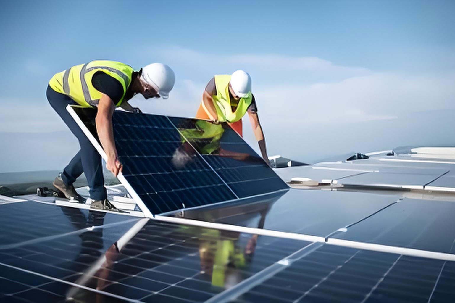
This plan deeply integrates intelligent diagnosis results with visualized operation and maintenance, significantly improving the efficiency and accuracy of fault localization and treatment.
System Deployment and Full‑Station Inspection
During deployment, I installed three edge servers in the station’s operation and maintenance center, each running a lightweight diagnostic model to handle data preprocessing and real‑time alarming, with an average response time ≤ 10 s. Simultaneously, a cloud data center and visualization platform were set up to achieve full‑station real‑time monitoring and fault visualization. After deployment, I conducted the first full‑station intelligent inspection. Traditional manual inspection of all 41,600 solar panels took about 48 hours, while the intelligent system, using drones equipped with infrared cameras and multi‑channel electrical parameter acquisition devices, completed the full scan in only 8 hours – an efficiency improvement of 83.3%. The inspection automatically identified 87 fault points, including 32 composite faults (20 hot spot + power degradation, 10 hot spot + poor connection, 6 power degradation + poor connection) and 55 single faults. The inspection report automatically generated a detailed list containing fault location, type, confidence, and treatment recommendations, providing precise guidance for subsequent verification and repair.
Performance Results
Through the application of the intelligent diagnosis and digital assisted treatment system, the station achieved remarkable operational and economic benefits. Key indicators before and after system deployment are compared in Table 2.
| Indicator | Before deployment | After deployment | Improvement |
|---|---|---|---|
| Annual generation efficiency | Baseline | Significant increase; fault area restored to design level | — |
| O&M staff | 8 people | 5 people | Reduced by 37.5% |
| Full‑station inspection cycle | Once per month | Once per quarter | Period extended by 3× |
| Annual O&M cost | Baseline | Reduced by 42.3% | Significant cost savings |
| Fault occurrence rate | Baseline | Reduced by over 85% | Reliability greatly enhanced |
The generation efficiency of the affected area was fully restored to historical levels. Intelligent inspection greatly improved work efficiency: the inspection cycle was extended from monthly to quarterly while maintaining full coverage and depth, and the maintenance team was reduced from 8 to 5 people. The annual operation and maintenance cost decreased by 42.3%, and the fault occurrence rate dropped by more than 85%.
Discussion and Future Prospects
The intelligent diagnosis model combining CNN, LSTM, and attention mechanism has proven effective for composite faults on solar panels in mountainous distributed stations. However, there is room for further improvement. I plan to explore the following directions:
- Transfer learning: To adapt the model to different site conditions and panel types with limited labeled data.
- Multi‑modal fusion: Incorporate additional data sources such as electroluminescence images or acoustic signals for even earlier fault detection.
- Edge‑cloud collaborative architecture: To reduce latency and bandwidth consumption while maintaining high diagnostic accuracy.
- Predictive maintenance: Use the attention‑weighted features to predict remaining useful life of solar panels and schedule proactive replacements.
In conclusion, the proposed framework has significantly improved the intelligence and economic efficiency of the station’s operation, providing a solid foundation for the reliable and sustainable operation of large‑scale photovoltaic plants.
| Component | Formulation |
|---|---|
| CNN convolution | $$\mathbf{F}^{(l)}_s = \sigma(\mathbf{W}^{(l)}_s * \mathbf{F}^{(l-1)}_s + \mathbf{b}^{(l)}_s)$$ |
| LSTM gates and state | $$\begin{aligned} i_t &= \sigma(\mathbf{W}_{xi}x_t + \mathbf{W}_{hi}h_{t-1} + b_i) \\ f_t &= \sigma(\mathbf{W}_{xf}x_t + \mathbf{W}_{hf}h_{t-1} + b_f) \\ o_t &= \sigma(\mathbf{W}_{xo}x_t + \mathbf{W}_{ho}h_{t-1} + b_o) \\ \tilde{C}_t &= \tanh(\mathbf{W}_{xc}x_t + \mathbf{W}_{hc}h_{t-1} + b_c) \\ C_t &= f_t \odot C_{t-1} + i_t \odot \tilde{C}_t \\ h_t &= o_t \odot \tanh(C_t) \end{aligned}$$ |
| Attention weight | $$e_i = \mathbf{v}_a^{\mathsf{T}} \tanh(\mathbf{W}_a \mathbf{h}_i + b_a), \quad \alpha_i = \frac{\exp(e_i)}{\sum_j \exp(e_j)}$$ |
| Attended feature | $$\mathbf{F}_{\text{att}} = \sum_i \alpha_i \mathbf{h}_i$$ |
| Softmax classification | $$p(y=k) = \frac{\exp(\mathbf{w}_k^{\mathsf{T}} \mathbf{F}_{\text{att}} + b_k)}{\sum_{c} \exp(\mathbf{w}_c^{\mathsf{T}} \mathbf{F}_{\text{att}} + b_c)}$$ |
By implementing this intelligent diagnostic system, I have demonstrated that advanced deep learning models, when properly integrated with digital twin and visualization technologies, can dramatically improve the fault diagnosis capability for solar panels in complex environments. The approach not only boosts accuracy and localization precision but also reduces operational costs and human effort, paving the way for fully autonomous photovoltaic plant management.