
The global pursuit of carbon peak and carbon neutrality goals has catalyzed an unprecedented acceleration in the development of clean energy. Among the various renewable options, solar photovoltaic (PV) technology has garnered significant attention. This momentum is supported by a dense array of policy documents issued at both national and local levels, actively promoting the adoption of photovoltaic systems. Municipal engineering projects, often characterized by large footprints and minimal surrounding obstructions, present ideal conditions for photovoltaic installations. In response to governmental advocacy, there is a growing trend to integrate solar power systems into such infrastructure. This article, drawn from my professional experience, details the design and application of a rooftop photovoltaic system for a bus parking and maintenance depot, covering fundamental knowledge, critical calculations, and system design considerations.
The project involves a bus depot facility primarily designed for the repair, inspection, and maintenance of public transit vehicles, with ancillary office functions. The total roof area available is 2,678 square meters. The facility’s estimated total electrical load is approximately 460 kW. The site is located in a region with coordinates at 114.21°E longitude and 30.25°N latitude, at an elevation of 23 meters. The building is oriented true north-south. Key meteorological data includes an extreme high temperature of 41.3°C and an extreme low of -18.1°C. The annual sunshine duration ranges from 1,810 to 2,100 hours, classifying the area as having relatively abundant solar resources, which is favorable for the deployment of a solar system.
The selection of photovoltaic modules is a foundational decision. The mainstream technologies are broadly categorized into crystalline silicon and thin-film. While thin-film cells offer advantages like flexibility and better performance in low-light or high-temperature conditions, the technology is not yet as mature or widely deployed at scale for such projects. Therefore, after considering conversion efficiency and cost, the polycrystalline silicon type within the crystalline silicon category was chosen. Furthermore, modules are available in single-glass and double-glass bifacial designs. Bifacial double-glass modules can improve photovoltaic conversion efficiency by 3% to 5% compared to standard single-glass panels by capturing reflected light on the rear side. With advances in manufacturing reducing the price differential, the bifacial double-glass polycrystalline silicon module was selected. The chosen panel dimensions are 2,278 mm in length and 1,134 mm in width, giving a single-panel area of approximately 2.583 m².
The choice of inverter is equally critical. The primary types are centralized and string inverters. A comparison of their key characteristics is essential for selection.
| Comparison Item | Centralized Inverter | String Inverter |
|---|---|---|
| Power Range | >500 kW | 3–320 kW |
| Protection Rating | Typically IP20 (requires indoor installation) | Typically IP65/66 (suitable for outdoor installation) |
| Flexibility & Configuration | Lower. Narrower MPPT voltage range. Cannot monitor individual strings closely. | High. Wider MPPT voltage range. Multiple independent MPPTs per inverter. |
| System Reliability | Lower. A single failure affects a large portion of the solar system. | Higher. Failure of one unit only affects its assigned strings. |
| Initial Cost | Generally lower per kW. | Slightly higher. |
| Energy Yield (Efficiency) | High, but can be reduced by string mismatch. | Very high, optimized per string. |
| Maintenance Cost | Lower, but downtime for repair can be significant. | Higher unit count, but easier and faster module-level replacement. |
Centralized inverters have a narrower Maximum Power Point Tracking (MPPT) voltage range and cannot monitor individual string performance closely, preventing each string from operating at its absolute optimal point. They are better suited for large, uniform installations like ground-mounted solar farms. For a medium-sized rooftop solar system like this depot, where the roof may have minor inhomogeneities and the scale is appropriate, string inverters offer superior flexibility, reliability, and energy harvest. Their higher protection rating also allows for decentralized mounting near the PV arrays, reducing DC cable lengths. Consequently, string inverters were selected for this project.
The electrical design of the solar system begins with determining the orientation and tilt angle of the PV modules. The building roof is oriented true north-south, which is optimal for maximizing solar irradiance capture in the northern hemisphere, corresponding to an azimuth angle of 0°. The theoretical optimum tilt angle (β) for this latitude (φ = 30.25°) to maximize annual yield is approximately equal to the latitude. However, practical adjustments are often made. For this project, based on solar resource data and the absence of shading from surrounding objects, a tilt angle of 22° was determined to be optimal.
A crucial calculation is the spacing between rows of PV modules to prevent shading, which would drastically reduce the solar system’s output. According to relevant design standards, the spacing should ensure no mutual shading between rows from 9:00 AM to 3:00 PM solar time. The required spacing (D) can be calculated using the following formulas, which account for the sun’s position at the winter solstice (typically the worst-case scenario for shading):
$$ B = L \times \cos \beta $$
$$ D = L \times \sin \beta \times \frac{0.707 \tan \alpha + 0.4338}{0.707 – 0.4338 \tan \alpha} $$
Where:
\( L \) = Length of the PV module (2278 mm)
\( \beta \) = Tilt angle (22°)
\( \alpha \) = Solar altitude angle for the design day. This is often derived from the latitude (φ). For the winter solstice, a common approximation is used where \( \tan \alpha \) relates to the latitude. The formula above incorporates constants for the sun’s position at 9 AM/3 PM solar time on December 21st.
For this location (φ ≈ 30.25°), the calculation yields a spacing \( D \) of approximately 1590 mm.
The projected length of a single module on the ground is \( B \), calculated as 2112 mm. The projected width remains the module width of 1134 mm.
The next step is determining the total installed area and capacity of the solar system. This project was designed concurrently with the main building, so detailed historical load curves were unavailable. Based on analogous projects, the minimum daytime load during spring and autumn was estimated to be around 200 kW. The sizing of this particular solar system was primarily area-driven, guided by local regulations mandating that the installed PV area should cover no less than 30% of the available roof area (excluding zones occupied by equipment and HVAC units).
Total available roof area: \( A_{roof} = 2678 \, m^2 \)
Minimum required PV area: \( A_{PV\_min} = A_{roof} \times 0.30 = 803.4 \, m^2 \)
This area refers to the total area occupied by the module frames, excluding the row spacing calculated earlier.
An initial estimate of the number of modules (N) is:
$$ N_{estimate} = \frac{A_{PV\_min}}{Area_{module}} = \frac{803.4}{2.583} \approx 311.03 $$
Rounded to 312 modules for preliminary calculation.
The rated power per module is 550 Wp. Therefore, the total preliminary DC capacity (\( P_{dc} \)) is:
$$ P_{dc} = N \times P_{module} = 312 \times 0.55 \, kW = 171.6 \, kWp $$
This capacity is below the estimated minimum load, indicating that the generated energy can be fully consumed on-site (high self-consumption rate), which is economically beneficial.
The configuration of the string inverter is governed by voltage constraints to ensure safe and efficient operation of the solar system. The key formulas involve the maximum input voltage and the MPPT voltage range of the inverter.
1. Maximum Voltage Limit (based on coldest temperature):
$$ N_{max} \leq \frac{V_{dcmax}}{V_{oc} \times [1 + (t_{min} – 25) \times K_v]} $$
2. MPPT Voltage Range Limit (based on operating temperatures):
$$ \frac{V_{mpptmin}}{V_{pm} \times [1 + (t_{max} – 25) \times K_v]} \leq N_{op} \leq \frac{V_{mpptmax}}{V_{pm} \times [1 + (t_{min} – 25) \times K_v]} $$
Where:
\( N \) = Number of modules in series.
\( V_{dcmax} \) = Inverter maximum DC input voltage (1100 V).
\( V_{oc} \) = Module open-circuit voltage (49.80 V).
\( V_{pm} \) = Module voltage at maximum power (41.95 V).
\( V_{mpptmin}, V_{mpptmax} \) = Inverter MPPT minimum and maximum voltages (160 V, 1000 V).
\( t_{min}, t_{max} \) = Record extreme low and high temperatures (-18.1°C, 41.3°C).
\( K_v \) = Module’s temperature coefficient for voltage (-0.265 %/°C = -0.00265 1/°C).
Performing the calculations:
For the maximum limit (cold):
$$ N_{max} \leq \frac{1100}{49.80 \times [1 + (-18.1 – 25) \times (-0.00265)]} = \frac{1100}{49.80 \times [1 + (-43.1) \times (-0.00265)]} $$
$$ = \frac{1100}{49.80 \times [1 + 0.114215]} = \frac{1100}{49.80 \times 1.114215} = \frac{1100}{55.488} \approx 19.82 $$
∴ \( N_{max} \leq 19 \) (rounded down for safety).
For the MPPT range:
Lower limit (at high temperature):
$$ N_{op} \geq \frac{160}{41.95 \times [1 + (41.3 – 25) \times (-0.00265)]} = \frac{160}{41.95 \times [1 + (16.3) \times (-0.00265)]} $$
$$ = \frac{160}{41.95 \times [1 – 0.043195]} = \frac{160}{41.95 \times 0.956805} = \frac{160}{40.138} \approx 3.99 $$
∴ \( N_{op} \geq 4 \).
Upper limit (at low temperature, within MPPT):
$$ N_{op} \leq \frac{1000}{41.95 \times [1 + (-18.1 – 25) \times (-0.00265)]} = \frac{1000}{41.95 \times 1.114215} = \frac{1000}{46.741} \approx 21.39 $$
∴ \( N_{op} \leq 21 \).
Combining the constraints: \( 4 \leq N \leq 19 \). For optimal performance, it is best for all strings connected to an inverter to have an identical number of modules. Considering inverter model capacity (50 kW), module power, and layout convenience, 13 modules per string was chosen. With each module at 0.55 kW, the DC power per string is 7.15 kW. A 50 kW inverter with 4 MPPT trackers, each supporting 2 strings, can accommodate 8 strings. The total DC capacity per inverter would be \( 8 \times 7.15 \, kW = 57.2 \, kW \), giving a DC-to-AC ratio (or inverter loading ratio) of \( 57.2 / 50 = 1.14 \), which is a common and efficient design practice for solar systems in this region. The total number of modules (312) divided by 8 strings per inverter indicates a need for \( 312 / 8 = 39 \) strings. This requires \( 39 / 2 \) (strings per MPPT) ≈ 20 MPPT channels, meaning multiple inverters. In the final design, the total system was divided among several 50 kW string inverters.
The physical layout of the solar system on the roof must account for shading obstructions. The perimeter parapet wall, with a height of 1 meter, creates shading zones at the edges. Using solar pathfinder software or trigonometric calculations, these no-go zones are mapped, typically appearing as fan-shaped areas at the roof corners. The PV arrays are then arranged within the unshaded central area, respecting the calculated row spacing (D). Inverters are mounted in clusters at accessible locations to minimize DC cabling losses and facilitate maintenance. The architectural drawing above provides a conceptual view of such a rooftop solar system layout, showing orderly rows of panels.
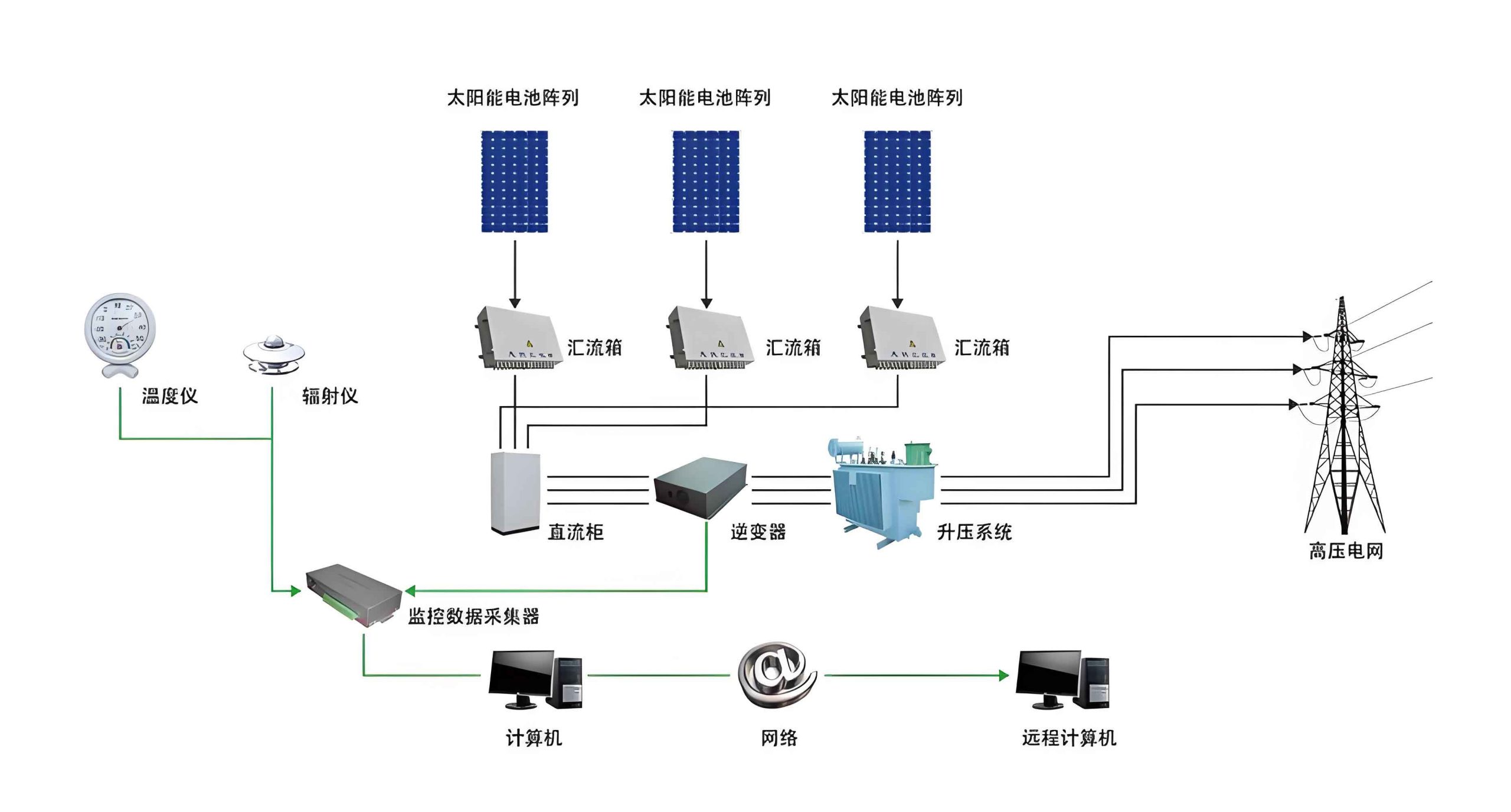
The system architecture is relatively straightforward for a project of this scale. The total installed DC capacity is 171.6 kWp. According to electrical standards, a low-voltage (400 V) grid connection is applicable for systems typically below a certain threshold (often around 500 kW). The PV strings are connected to their designated string inverters. The AC outputs of these inverters are then combined in a common AC combiner/distribution panel before being fed into a dedicated grid-connection cabinet located in the main substation room. A simplified single-line diagram illustrates this: PV Arrays → String Inverters → AC Combiner Panel → Grid-Connection Cabinet → Facility’s Main Low-Voltage Switchboard.
A critical requirement for grid-connected solar systems is protection against “islanding.” Islanding occurs when a distributed generator, like our PV system, continues to power a section of the network after grid power has been lost. This can be dangerous for utility workers and may damage equipment due to unstable voltage and frequency. Modern string inverters come equipped with active anti-islanding protection that continuously monitors grid parameters and shuts down if the grid fails. Additionally, the grid connection agreement often requires a separate grid monitoring relay at the point of common coupling for added security, ensuring the solar system disconnects reliably during a grid outage.
Furthermore, a comprehensive monitoring system is implemented. This system collects data from each inverter—such as AC power output, energy yield, operating status, and fault logs—and transmits it to a local display and/or a cloud-based platform. This allows for real-time performance assessment, prompt fault detection, and yield analysis of the entire solar system, ensuring optimal long-term operation and return on investment.
Finally, estimating the annual energy yield (Ep) of the solar system is essential for economic and environmental assessments. A standard formula is used:
$$ E_p = H_A \times \frac{P_{AZ}}{E_S} \times K $$
Where:
\( H_A \) = Annual total solar irradiation on the horizontal plane (kWh/m²). For the project location, this value is obtained from meteorological databases or simulation software (e.g., PVGIS). Assume \( H_A \) = 1238.6 kWh/m².
\( P_{AZ} \) = Total installed PV array capacity at STC = 171.6 kWp.
\( E_S \) = Standard irradiance (1 kW/m²).
\( K \) = Overall system performance ratio (a dimensionless coefficient accounting for all losses).
The performance ratio (K) encompasses losses from:
• Temperature effects on modules
• Soiling (dirt on panels)
• Wiring and connection losses (DC & AC)
• Inverter efficiency
• Transformer losses (if any)
• Shading (minimized by design)
• Module mismatch and degradation
A typical value for a well-designed, commercial rooftop solar system is around 0.75 to 0.85. For this calculation, we assume \( K = 0.80 \).
Substituting the values:
$$ E_p = 1238.6 \, \text{kWh/m}^2 \times \frac{171.6 \, \text{kWp}}{1 \, \text{kW/m}^2} \times 0.80 $$
$$ E_p = 1238.6 \times 171.6 \times 0.80 $$
$$ E_p \approx 170,000 \, \text{kWh/year} $$
This estimated annual production of 170 MWh represents a significant portion of the depot’s energy consumption, contributing directly to reduced grid electricity purchases and lower operational carbon emissions.
In conclusion, the integration of a solar photovoltaic system into a bus depot facility is a technically viable and strategically sound project that aligns with broader sustainability goals. The design process involves careful selection of components—opting for bifacial modules and string inverters in this case—followed by precise engineering calculations to determine optimal tilt, spacing, string configuration, and overall capacity. The layout must carefully avoid shading obstructions. The final grid-connected system requires robust protection against islanding and a monitoring system for performance management. This case study demonstrates how a methodical approach, from policy-driven area targets to detailed electrical calculations, can result in an efficient and reliable on-site solar power generation system. The principles outlined here—sizing based on available area and policy, meticulous component selection, and adherence to electrical and safety standards—provide a framework for the successful implementation of solar systems in similar municipal and industrial infrastructure projects.