
Photovoltaic power generation has become a cornerstone of the global clean energy transition. The efficiency and safety of solar power plants depend critically on the operational condition of solar panels, which are exposed to harsh outdoor environments for decades. Defects such as hotspots, micro-cracks, dust accumulation, and bird droppings can significantly reduce energy yield and even cause permanent damage. Traditional manual inspection methods are labor-intensive, subjective, and inadequate for large-scale photovoltaic farms. Deep learning-based object detection offers a promising solution for automated defect identification, yet challenges remain in terms of detection accuracy, generalization, and real-time performance in complex scenes. In this thesis, I focus on algorithmic improvements and system implementation to construct an efficient and reliable intelligent detection system for solar panel surface defects. I first build a high-quality dataset containing six typical categories: clean, physical damage, electrical damage, dust, snow, and bird droppings. Then I propose two-stage model optimization strategies based on improved YOLOv5s and YOLOv8s architectures. Finally, I develop a complete PyQt5-based software system that integrates the improved algorithms for practical inspection. Extensive experiments demonstrate that the proposed methods achieve superior detection accuracy while maintaining real-time inference speed, providing solid technical support for intelligent operation and maintenance of solar power plants.
1. Introduction and Background
The increasing reliance on fossil fuels has led to severe environmental pollution and global climate change. The combustion of coal, oil, and natural gas releases pollutants such as sulfur dioxide, nitrogen oxides, and particulate matter, as well as massive amounts of greenhouse gases, especially carbon dioxide. According to the International Energy Agency (IEA), the vast majority of global greenhouse gas emissions originate from fossil fuel combustion. To mitigate these effects, international communities have set ambitious carbon neutrality targets. Renewable energy sources, particularly solar energy, are key to achieving these goals. In China, the photovoltaic (PV) industry has grown rapidly. By the end of 2024, the cumulative installed capacity of solar power reached a staggering level, with annual additions exceeding 100 GW since 2021. The share of solar PV in renewable energy generation capacity continues to rise, as illustrated by the data showing that solar PV contributed about 70% of the new renewable capacity worldwide in 2024.
However, the operation and maintenance of photovoltaic plants face significant challenges. Solar panels are installed in diverse environments, from deserts and plains to rooftops and even offshore areas. They are subjected to various external factors that lead to different types of defects. Among them, hotspot effect is a major concern, caused by partial shading, dust, bird droppings, or internal circuit faults, which result in local temperature rises and permanent damage. Regular inspection is essential to ensure optimal performance and safety. Traditional inspection methods, such as manual visual inspection or thermal imaging by human operators, are inefficient and often miss early subtle defects. The use of unmanned aerial vehicles (UAVs) equipped with cameras has improved coverage, but the analysis of large volumes of imagery still relies heavily on manual interpretation, which is subjective and error-prone. Therefore, an intelligent, automated, and accurate defect detection system for solar panels is of great practical importance.
Recent advances in deep learning, especially convolutional neural networks (CNNs) and object detection algorithms, have opened new avenues for automated visual inspection. Object detection frameworks can localize and classify defects in images simultaneously. Two-stage detectors, such as Faster R-CNN, offer high accuracy but are slow; one-stage detectors, such as the You Only Look Once (YOLO) series, have achieved an excellent trade-off between speed and accuracy, making them suitable for real-time applications. In this work, I focus on improving YOLO-based models specifically for solar panel surface defect detection. The main contributions of this thesis are summarized as follows:
- Construction of a high-quality solar panel defect dataset consisting of six categories, with comprehensive data augmentation techniques.
- Proposal of an improved YOLOv5s model incorporating DynamicConv, iRMB attention, and HATHead detection head, which significantly boosts detection accuracy and recall.
- Development of a lightweight improved YOLOv8s algorithm integrating C2f-SENetV2, EMA attention, and Inner-ShapeIOU loss, achieving a superior balance between precision and speed.
- Implementation of a complete PyQt5-based defect detection system with modules for detection, visualization, and result saving, supporting image, video, and real-time camera inputs.
2. Related Work and Theoretical Foundations
2.1 Convolutional Neural Networks
Convolutional Neural Networks (CNNs) are the backbone of modern object detection. A typical CNN consists of convolutional layers, activation functions, pooling layers, and fully connected layers. The convolutional layer extracts local features using learnable kernels. The activation function introduces nonlinearity. Commonly used activation functions include Sigmoid, Tanh, and ReLU. The Sigmoid function is defined as:
$$f(x) = \frac{1}{1 + e^{-x}}$$
The Tanh function is:
$$f(x) = \frac{e^x – e^{-x}}{e^x + e^{-x}}$$
The ReLU function is:
$$f(x) = \max(0, x)$$
Pooling layers reduce spatial dimensions, providing translation invariance and reducing computational load. Fully connected layers map extracted features to final outputs. Architectures such as VGG, ResNet, and CSPNet have evolved to improve feature extraction and gradient flow.
2.2 Object Detection Algorithms
Object detection aims to identify and classify objects while localizing them with bounding boxes. Two-stage algorithms, including R-CNN, Fast R-CNN, and Faster R-CNN, follow a region-proposal paradigm. They first generate candidate regions and then classify and refine them. While accurate, they suffer from high computational cost. In contrast, one-stage algorithms such as SSD and YOLO directly predict classes and locations from feature maps in a single pass, offering high speed. The YOLO series has evolved through several versions, from YOLOv1 to YOLOv8. YOLOv1 treats detection as a regression problem. YOLOv3 introduced multi-scale prediction with feature pyramid networks. YOLOv5 and YOLOv8 are widely used in industrial applications due to their balanced performance. YOLOv8 features an anchor-free head and C2f modules, which improve efficiency and representational power.
2.3 Attention Mechanisms
Attention mechanisms enable neural networks to focus on important features and suppress irrelevant ones. SENet applies channel-wise attention by squeezing global spatial information and exciting channel dependencies. CBAM combines channel and spatial attention. ECA uses a lightweight 1D convolution for channel attention, achieving efficiency. These mechanisms have been successfully integrated into detection backbones to boost performance.
2.4 Evaluation Metrics
Common evaluation metrics for object detection include precision (P), recall (R), average precision (AP), mean average precision (mAP), and frames per second (FPS). IoU measures the overlap between predicted and ground-truth boxes. Precision and recall are defined as:
$$P = \frac{TP}{TP + FP}, \quad R = \frac{TP}{TP + FN}$$
mAP is the mean of AP over all classes. Higher mAP indicates better detection performance, while FPS indicates real-time capability.
3. Dataset Construction and Preprocessing
3.1 Defect Types
The performance of deep learning models heavily depends on the quality and diversity of the training data. Publicly available annotated datasets for solar panel defects are scarce. Therefore, I constructed a custom dataset by collecting images from real PV plants and online open-source resources. The dataset covers six typical surface conditions:
- Clean – panels in normal operating condition.
- Physical damage – cracks, fractures caused by hail or mechanical stress.
- Electrical damage – hotspots, burn marks, and potential-induced degradation.
- Dust – accumulation of dust particles on the panel surface.
- Snow – snow coverage blocking sunlight.
- Bird droppings – local shading and chemical corrosion.
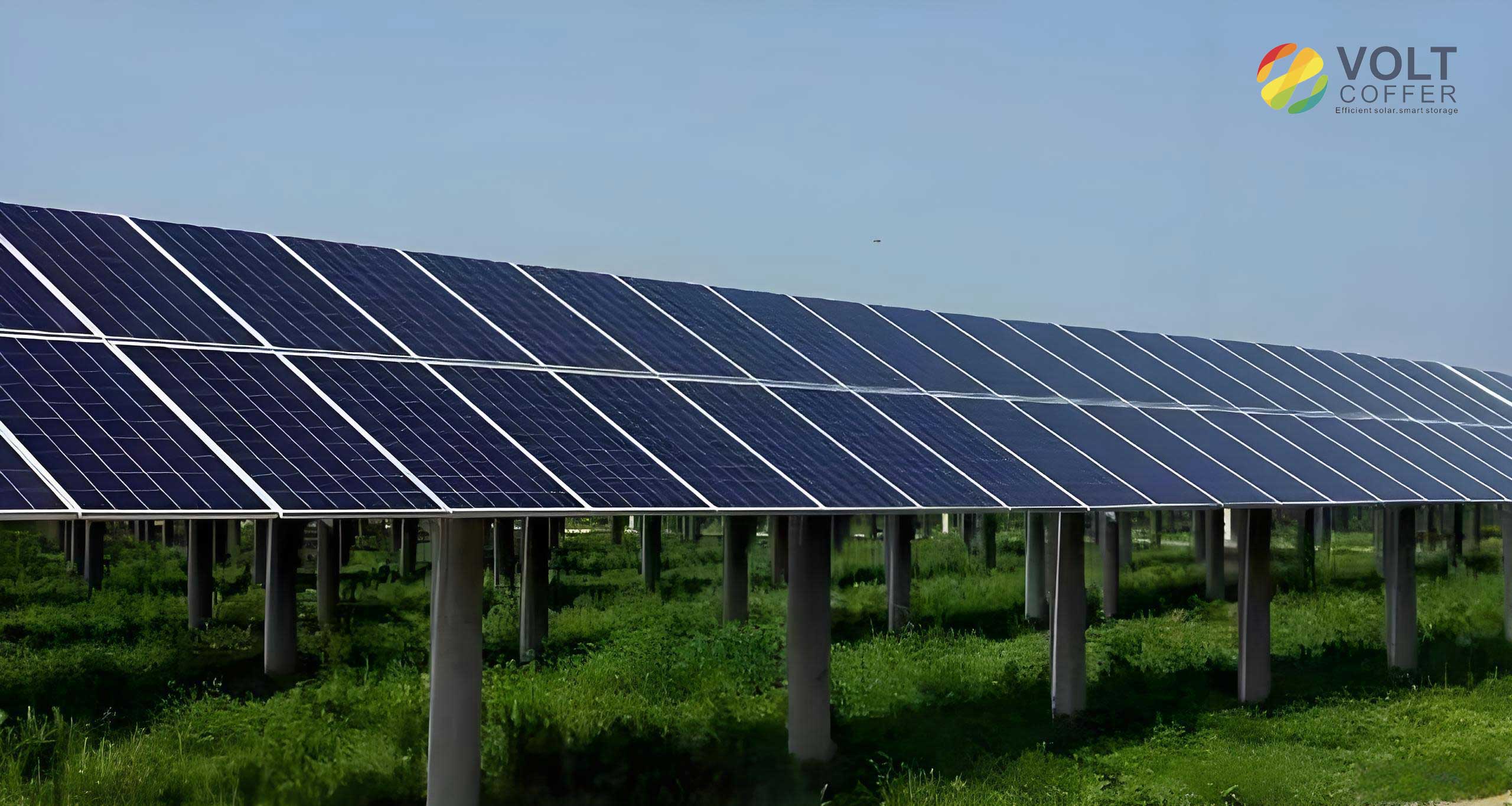
Figure above illustrates a typical solar panel installation, which is subject to various environmental factors. Accurate detection of these defect types is essential for timely maintenance.
3.2 Image Preprocessing
Raw images often contain background noise and irrelevant regions. I applied effective region extraction to isolate the solar panel area. Since solar panels have distinct texture and color from their surroundings, a texture-based segmentation method was employed. The average RGB value and contrast mean were used to improve extraction accuracy. After cropping the panel region, Gaussian filtering was applied to remove noise while preserving defect features. The processed images were then annotated using the LabelImg tool, producing bounding boxes and class labels in TXT format.
3.3 Data Augmentation
To improve generalization and mitigate overfitting, I applied geometric transformations including horizontal flip, vertical flip, random scaling, random shearing, and perspective transformation. In addition, Mosaic data augmentation was adopted. Mosaic randomly selects four training images, scales them, and stitches them into one composite image. This enriches the context and enhances multi-object detection capabilities. After augmentation, the final dataset contained 14,478 images, which were split into training (80%), validation (10%), and test (10%) subsets, resulting in 11,582 training images, 1,448 validation images, and 1,448 test images.
4. Improved YOLOv5s for Solar Panel Defect Detection
4.1 Baseline YOLOv5s
YOLOv5s is a lightweight version of the YOLOv5 series, containing about 7.2 million parameters. Its architecture comprises an input stage, a backbone (CSPDarknet), a neck (PANet), and a detection head. The backbone uses Focus and C3 modules. The SPP layer expands the receptive field. The neck uses a feature pyramid network to fuse multi-scale features. The detection head predicts bounding boxes and class probabilities. However, the standard YOLOv5s has limitations in detecting small and subtle defects on solar panels due to insufficient contextual and multi-scale information.
4.2 Dynamic Convolution
To reduce computational complexity while maintaining high feature representation, I replaced the standard convolutions in the backbone with DynamicConv. DynamicConv generates convolution kernels conditioned on the input, allowing the network to adaptively fuse multiple expert kernels. The standard convolution operation can be expressed as:
$$Y = X * W$$
where \(X\) is the input and \(W\) is the static kernel. DynamicConv instead computes a dynamic weight \(W’\) by a linear combination of \(M\) expert kernels \(W_i\) with input-dependent coefficients \(\alpha_i\):
$$W’ = \sum_{i=1}^{M} \alpha_i W_i$$
The coefficients are generated by a two-layer MLP followed by softmax:
$$\alpha = \text{softmax}(\text{MLP}(\text{Pool}(X)))$$
DynamicConv increases the parameter count and model capacity without a significant increase in FLOPs because the kernel combination is performed on a small set. As shown in the experiments, it improves the accuracy by 1.1% mAP0.5 over the baseline while preserving real-time speed.
4.3 iRMB Attention Mechanism
To enhance the perception of subtle defects, I integrated the iRMB (inverted Residual Mobile Block) attention mechanism into the feature pyramid network. iRMB combines depthwise convolution (DW-Conv) with an efficient window-based multi-head self-attention (EW-MHSA). The input feature \(X \in \mathbb{R}^{C \times H \times W}\) is first expanded to \(X_e\) via a fully connected layer:
$$X_e = \text{MLP}_e(X) \in \mathbb{R}^{\lambda C \times H \times W}$$
where \(\lambda > 1\) is the expansion factor. The attention matrix is computed from the original feature \(X\) (query and key) while the value comes from the expanded feature \(X_e\):
$$Q = K = \text{Linear}(X), \quad V = X_e$$
$$\text{Attn}(X_e) = \text{Softmax}\left(\frac{Q K^T}{\sqrt{d}}\right) \cdot V$$
Then a depthwise convolution extracts local details:
$$X_f = \text{DW-Conv}(\text{Attn}(X_e))$$
Finally, the output is fused with the input via a residual connection:
$$Y = X + \text{MLP}_s(X_f)$$
This module improves the ability to capture long-range dependencies while keeping computation low. The inclusion of iRMB increased recall by 5.5% when used alone, although it reduced FPS due to the added computation.
4.4 HATHead Detection Head
The original detection head was replaced with HATHead, which is designed based on the Hybrid Attention Transformer (HAT) architecture. HATHead combines channel attention and spatial self-attention in a Hybrid Attention Block (HAB) and further incorporates overlapping cross-attention blocks to model global context. The hybrid attention adaptively recalibrates features across both channels and spatial positions. This structure enhances the sensitivity to small-scale defects and improves multi-scale localization. By replacing the head, recall increased to 85.4% and mAP0.5 to 89.4%, while maintaining a high FPS of 141.
4.5 Experiments and Results
4.5.1 Experimental Setup
All experiments were conducted on a workstation with Windows 11, an NVIDIA RTX 4060 GPU with 8 GB memory, Python 3.8.5, PyTorch 1.9.0, and CUDA 11.6. The input image size was 640 pixels, batch size was 16, and the training ran for 200 epochs. The SGD optimizer was used with an initial learning rate of 0.01, momentum of 0.937, and weight decay of 0.0005. The hyperparameters are summarized in the table below.
| Hyperparameter | Value |
|---|---|
| image-size | 640 |
| epochs | 200 |
| batch | 16 |
| workers | 0 |
| device | 0 |
| optimizer | SGD |
| amp | True |
| lr0 | 0.01 |
| momentum | 0.937 |
| weight-decay | 0.0005 |
4.5.2 Comparison of Convolution Modules
I conducted experiments to compare different convolution modules in the backbone. The results are shown in Table 2.
| Convolution | P/% | R/% | mAP0.5/% | mAP0.5:0.95/% | FPS |
|---|---|---|---|---|---|
| ODConv | 80.5 | 79.2 | 84.4 | 84.3 | 133 |
| SAConv | 83.9 | 80.7 | 86.5 | 86.4 | 111 |
| RFAConv | 82.7 | 77.2 | 84.7 | 84.6 | 89 |
| DynamicConv | 84.4 | 79.2 | 87.7 | 87.7 | 143 |
DynamicConv achieved the highest mAP0.5 (87.7%) and the highest FPS (143), demonstrating a good balance between accuracy and speed. SAConv had the best recall (80.7%) among the compared modules, suggesting its strength in detecting positive defects, but its FPS was lower. Therefore, DynamicConv was selected as the backbone convolution.
4.5.3 Comparison of Detection Heads
I also compared different detection head modules. Table 3 shows the results.
| Head | P/% | R/% | mAP0.5/% | mAP0.5:0.95/% | FPS |
|---|---|---|---|---|---|
| RepHead | 85.2 | 80.2 | 88.5 | 88.4 | 135 |
| SAHead | 79.9 | 83.6 | 87.9 | 87.9 | 133 |
| HATHead | 81.9 | 85.4 | 89.4 | 89.4 | 141 |
| FRMHead | 88.1 | 75.5 | 87.3 | 87.2 | 92 |
HATHead achieved the highest recall (85.4%) and the best mAP0.5 (89.4%), showing its advantage in detecting defects comprehensively. Although FRMHead had the highest precision (88.1%), its very low recall (75.5%) and FPS (92) make it unsuitable for real-time inspection. HATHead offers the best comprehensive performance and thus was adopted.
4.5.4 Ablation Study
To evaluate the contribution of each module, I performed ablation experiments by incrementally adding DynamicConv, HATHead, and iRMB to the baseline YOLOv5s. The results are presented in Table 4.
| YOLOv5s | DynamicConv | HATHead | iRMB | P/% | R/% | mAP0.5/% | mAP0.5:0.95/% | FPS |
|---|---|---|---|---|---|---|---|---|
| ✓ | — | — | — | 85.5 | 77.9 | 86.6 | 86.5 | 147 |
| ✓ | ✓ | — | — | 84.4 | 79.2 | 87.7 | 87.7 | 143 |
| ✓ | — | ✓ | — | 81.9 | 85.4 | 89.4 | 89.4 | 141 |
| ✓ | — | — | ✓ | 80.7 | 83.4 | 87.4 | 87.3 | 101 |
| ✓ | ✓ | ✓ | — | 89.1 | 79.7 | 88.4 | 88.4 | 137 |
| ✓ | — | ✓ | ✓ | 88.5 | 81.9 | 89.6 | 89.6 | 91 |
| ✓ | ✓ | — | ✓ | 88 | 81.6 | 87.5 | 87.5 | 96 |
| ✓ | ✓ | ✓ | ✓ | 81.3 | 87.5 | 90.2 | 90.1 | 90 |
The full integration of all three modules produced the highest recall (87.5%) and mAP0.5 (90.2%), confirming that the modules complement each other. HATHead contributed most significantly to improving recall and accuracy, while DynamicConv maintained efficiency, and iRMB further improved coverage at the cost of speed.
4.5.5 Comparison with Other Models
I compared the improved YOLOv5s with several official YOLO versions and recent models. The results are shown in Table 5.
| Model | P/% | R/% | mAP0.5/% | mAP0.5:0.95/% | FPS |
|---|---|---|---|---|---|
| YOLOv5n | 80.5 | 78.8 | 84.8 | 84.7 | 294 |
| YOLOv5s | 85.5 | 77.9 | 86.6 | 86.5 | 147 |
| YOLOv5m | 82.9 | 79.2 | 86.3 | 86.3 | 68 |
| YOLOv5l | 82.5 | 83.3 | 86.9 | 86.8 | 52 |
| YOLOv9s | 84.8 | 74.4 | 85.1 | 85 | 125 |
| YOLOv11s | 83.7 | 80.4 | 88.5 | 88 | 138 |
| Improved YOLOv5 | 81.3 | 87.5 | 90.2 | 90.1 | 90 |
The improved YOLOv5 achieved the highest mAP0.5 and mAP0.5:0.95 among all compared models, with a significant improvement over the baseline YOLOv5s (90.2% vs 86.6% mAP0.5). Although its FPS of 90 is lower than the tiny versions, it still meets real-time requirements. This demonstrates the effectiveness of the proposed improvements.
5. Lightweight Improved YOLOv8s
5.1 Baseline YOLOv8s
While the improved YOLOv5s achieved high accuracy, its network structure is relatively shallow and may not fully exploit multi-scale and fine-grained features. To further break the performance limit and achieve a better speed-accuracy trade-off, I turned to YOLOv8s, which introduces an anchor-free detection head, C2f modules, and dynamic label assignment. YOLOv8s offers a more modern architecture that naturally supports multi-scale and multi-category detection tasks. However, to specialize it for solar panel defect detection, I proposed three key improvements: embedding a lightweight SENetV2 channel attention into the C2f module, introducing the EMA multi-scale attention module in the neck, and adopting the Inner-ShapeIoU loss function for precise bounding box regression.
5.2 C2f-SENetV2 Module
The C2f module in YOLOv8s splits the input feature map into two streams and concatenates them after passing through multiple bottleneck blocks. To enhance channel discrimination, I integrated SENetV2 into the C2f module, creating C2f-SENetV2. SENetV2 features a Squeeze aggregated Excitation (SaE) unit. The squeeze operation uses global average pooling to compress each channel into a scalar. The excitation operation employs multiple parallel fully connected branches to capture richer global context, then fuses their outputs. The reweighting applies the learned channel weights to the original features. This mechanism adaptively emphasizes important channels and suppresses irrelevant ones, thereby improving the model’s ability to distinguish defects from complex backgrounds. The structure significantly boosts recall by 4.5% (as shown in ablation), while maintaining a negligible impact on FPS.
5.3 EMA Attention Module
In the neck network, I introduced the Efficient Multi-scale Attention (EMA) module. EMA divides input features into groups and applies three parallel sub-networks: two 1D branches (one horizontal, one vertical) capture long-range dependencies, and one 3×3 branch captures local cross-channel interactions. The outputs are combined using cross-spatial learning and Sigmoid activation. Formally, for a feature group \(X_c \in \mathbb{R}^{C/G \times H \times W}\), the horizontal and vertical pooled features are computed as:
$$Z_c^{(H)}(H) = \frac{1}{W}\sum_{i=0}^{W-1} X_c(H, i)$$
$$Z_c^{(W)}(W) = \frac{1}{H}\sum_{j=0}^{H-1} X_c(j, W)$$
These pooled features are concatenated and passed through a shared 1×1 convolution to obtain a compact representation. The module then generates spatial attention weights via softmax and matrix multiplication, effectively fusing local and global contexts. EMA enables the neck to better aggregate features of different scales, improving detection robustness for defects of varying sizes.
5.4 Inner-ShapeIoU Loss
The default CIoU loss has a known issue of gradient vanishing when bounding boxes share the same aspect ratio but differ in size. To overcome this, I designed a combined loss function, Inner-ShapeIoU, which integrates ShapeIoU and InnerIoU. ShapeIoU considers the shape similarity between predicted and ground-truth boxes:
$$ww = \frac{2 \times (w^{gt})^{scale}}{(w^{gt})^{scale} + (h^{gt})^{scale}}$$
$$hh = \frac{2 \times (h^{gt})^{scale}}{(w^{gt})^{scale} + (h^{gt})^{scale}}$$
$$distance_{shape} = hh \times \frac{(x_c – x_c^{gt})^2}{c^2} + ww \times \frac{(y_c – y_c^{gt})^2}{c^2}$$
$$\Omega_{shape} = \left(1 – e^{-\frac{|w – w^{gt}|}{\max(w, w^{gt})}}\right)^\theta + \left(1 – e^{-\frac{|h – h^{gt}|}{\max(h, h^{gt})}}\right)^\theta$$
$$L_{ShapeIoU} = 1 – IoU + distance_{shape} + 0.5 \times \Omega_{shape}$$
InnerIoU computes IoU using an auxiliary smaller bounding box inside the predicted and ground-truth boxes, controlled by a ratio. The combined loss is:
$$L_{Inner-ShapeIoU} = L_{ShapeIoU} + IoU – IoU_{inner}$$
This formulation provides more detailed gradient signals, especially for small defects, thereby improving localization accuracy and model convergence.
5.5 Experiments and Results
5.5.1 C2f Module Comparison
I compared different C2f variants by replacing the standard C2f with various improved modules. Table 6 presents the results.
| C2f module | P/% | R/% | mAP0.5/% | mAP0.5:0.95/% | FPS |
|---|---|---|---|---|---|
| C2f-AKConv | 82.9 | 79.1 | 87.1 | 86.3 | 200 |
| C2f-FasterBlock | 80.4 | 83 | 87.2 | 87.1 | 141 |
| C2f-DFF | 86.6 | 80.1 | 89.3 | 89.2 | 135 |
| C2f-SENetV2 | 81.2 | 88.1 | 90.2 | 90.2 | 135 |
| C2f-iEMA | 83.7 | 85.6 | 89.5 | 89.5 | 123 |
| C2f-WTConv | 83.4 | 82.8 | 89.4 | 89.4 | 118 |
C2f-SENetV2 achieved the highest recall (88.1%) and competitive mAP0.5 (90.2%), while maintaining a reasonable FPS of 135. This confirms that SERetV2’s channel attention effectively enhances feature extraction for solar panel defects.
5.5.2 Loss Function Comparison
I first determined the optimal scale for ShapeIoU and ratio for InnerIoU. Tables 7 and 8 show the results.
| Model | P/% | R/% | mAP0.5/% | mAP0.5:0.95/% |
|---|---|---|---|---|
| ShapeIoU(scale=0) | 81 | 84.1 | 89.5 | 89.5 |
| ShapeIoU(scale=0.5) | 85.8 | 82.4 | 88.8 | 88.7 |
| ShapeIoU(scale=1) | 86.7 | 85.6 | 89.8 | 89.8 |
| ShapeIoU(scale=1.5) | 81.1 | 85.8 | 88.7 | 88.6 |
The best scale was 1, which gave the highest precision and mAP. For InnerIoU, the results are:
| Model | P/% | R/% | mAP0.5/% | mAP0.5:0.95/% |
|---|---|---|---|---|
| InnerIoU(ratio=0.5) | 87.5 | 87.9 | 90.2 | 90.2 |
| InnerIoU(ratio=0.7) | 85.5 | 80.5 | 89.1 | 89 |
| InnerIoU(ratio=1) | 80.3 | 82.3 | 89.9 | 89.8 |
| InnerIoU(ratio=1.2) | 86.8 | 85.8 | 89.8 | 89.8 |
| InnerIoU(ratio=1.5) | 79.4 | 85.6 | 89.6 | 89.5 |
Ratio=0.5 performed the best across all metrics, so it was chosen for the combined loss. Then I compared various loss functions, as shown in Table 9.
| Loss | P/% | R/% | mAP0.5/% | mAP0.5:0.95/% | FPS |
|---|---|---|---|---|---|
| CIoU | 82.6 | 83.6 | 89.4 | 89.3 | 137 |
| WIoU | 82.2 | 85.1 | 89 | 89 | 217 |
| EIoU | 83.1 | 80.6 | 90.2 | 90.2 | 222 |
| ShapeIoU | 86.7 | 84.1 | 89.5 | 89.5 | 135 |
| InnerIoU | 85.5 | 80.5 | 89.1 | 89 | 137 |
| Inner-ShapeIoU | 87.2 | 83.6 | 90.5 | 90.5 | 137 |
Inner-ShapeIoU achieved the highest precision (87.2%) and mAP0.5 (90.5%), demonstrating its superiority in optimizing the bounding box regression for this dataset. Its FPS is identical to CIoU, confirming that the loss function does not introduce extra computation.
5.5.3 Ablation Study for Improved YOLOv8s
I performed ablation experiments to analyze the contribution of C2f-SENetV2, EMA, and Inner-ShapeIoU. The results are shown in Table 10.
| YOLOv8s | C2f-SENetV2 | Inner-ShapeIoU | EMA | P/% | R/% | mAP0.5/% | mAP0.5:0.95/% | FPS |
|---|---|---|---|---|---|---|---|---|
| ✓ | — | — | — | 82.6 | 83.6 | 89.4 | 89.3 | 137 |
| ✓ | ✓ | — | — | 81.2 | 88.1 | 90.2 | 90.2 | 135 |
| ✓ | — | ✓ | — | 87.2 | 83.6 | 90.5 | 90.5 | 137 |
| ✓ | — | — | ✓ | 90.1 | 80.4 | 90.1 | 90.1 | 119 |
| ✓ | ✓ | ✓ | — | 84 | 85.3 | 90.1 | 90 | 135 |
| ✓ | — | ✓ | ✓ | 86.5 | 80.4 | 89.8 | 89.8 | 119 |
| ✓ | ✓ | — | ✓ | 80.5 | 86.3 | 90.8 | 90.8 | 116 |
| ✓ | ✓ | ✓ | ✓ | 88.3 | 81.7 | 92.1 | 91.8 | 116 |
The full model attained the best mAP0.5 (92.1%) and mAP0.5:0.95 (91.8%), confirming that all three modules positively contribute to performance. C2f-SENetV2 significantly boosts recall, Inner-ShapeIoU improves precision, and EMA enhances multi-scale feature expression. The final FPS of 116 is sufficient for real-time deployment.
5.5.4 Model Comparison
Finally, I compared the improved YOLOv8s with several mainstream models and with the improved YOLOv5s from the previous chapter. Table 11 presents the comprehensive comparison.
| Model | P/% | R/% | mAP0.5/% | mAP0.5:0.95/% | FPS |
|---|---|---|---|---|---|
| YOLOv6n | 76.8 | 82.5 | 85.6 | 85.6 | 217 |
| YOLOv6s | 77.8 | 84.5 | 86.5 | 86.5 | 141 |
| YOLOv6m | 74.5 | 83.6 | 84.7 | 84.7 | 52 |
| YOLOv6l | 74.5 | 80.1 | 84.3 | 84 | 34 |
| YOLOv8n | 83.4 | 81.8 | 89 | 88.9 | 270 |
| YOLOv8s | 82.6 | 83.6 | 89.4 | 89.3 | 137 |
| YOLOv8m | 84.1 | 81.1 | 89.3 | 89.3 | 62 |
| YOLOv8l | 81.6 | 82.2 | 89.2 | 89.2 | 45 |
| YOLOv8s-p2 | 81.3 | 83.1 | 89 | 88.9 | 85 |
| YOLOv8s-p6 | 81.8 | 73.7 | 82.2 | 82.2 | 141 |
| YOLOv8s-ghost | 83 | 81.1 | 87.5 | 87.4 | 159 |
| YOLOv9s | 84.8 | 74.4 | 85.1 | 85 | 125 |
| YOLOv11s | 83.7 | 80.4 | 88.5 | 88 | 138 |
| Improved YOLOv5 | 81.3 | 87.5 | 90.2 | 90.1 | 90 |
| Improved YOLOv8 | 88.3 | 81.7 | 92.1 | 91.8 | 116 |
The improved YOLOv8 outperforms all other models, achieving the highest precision (88.3%), mAP0.5 (92.1%), and mAP0.5:0.95 (91.8%). It also has a higher FPS than the improved YOLOv5 (116 vs 90), demonstrating excellent efficiency. This makes it the final algorithm for the developed detection system.
6. System Design and Implementation
6.1 System Requirements
To bridge the gap between algorithmic research and practical application, I designed and implemented a solar panel defect detection software system based on the improved YOLOv8s model. The system requirements include:
- Defect recognition: Automatically detect and classify typical defects on solar panels with high accuracy.
- Result visualization: Display annotated images with bounding boxes, class labels, confidence scores, and location coordinates.
- Result saving: Save detection records (original images, annotated results, defect data) for future analysis and traceability.
- Multiple input sources: Support image files, video files, and real-time camera feeds.
6.2 System Architecture
The system is developed using PyQt5 for the graphical user interface. It consists of three major modules:
- Detection module: Loads the trained model and performs inference on input images or frames. It handles image loading, model initialization, and running detection.
- Visualization module: Displays the annotated results, including a table listing defect types, positions, confidences, and other relevant metadata.
- Result saving module: Saves the detection outcomes to disk in structured formats, enabling historical data management.
6.3 User Interface
The main interface is divided into two areas: the image display area and the data display area. In the upper right, users can choose to load a single image, a folder of images, a video file, or open a camera. After clicking “Run”, the system processes the input and shows the annotated image with detected defect boxes. The lower right panel displays structured information for each detected object, including index, category, image name, timestamp, recognition result, number of targets, and save path. The parameter panel on the left shows the confidence and coordinates for the selected defect.
6.4 Functionality Test
I tested the system on images representing all six categories. The system accurately identified clean panels, physical damage, electrical damage, dust, snow, and bird droppings, displaying the correct class labels and confidence values. The detection results were correctly visualized and saved. The system runs smoothly and meets the real-time requirements for solar panel inspection.
7. Conclusion and Future Work
In this thesis, I addressed the challenge of intelligent defect detection for solar panels by proposing two improved YOLO-based models and an application system.
First, I constructed a comprehensive dataset with six defect categories and applied data augmentation to enhance diversity. Then, I proposed an improved YOLOv5s model incorporating DynamicConv, iRMB attention, and HATHead. Experiments showed that these modules improve detection accuracy and recall significantly. To further pursue a better trade-off between accuracy and speed, I developed a lightweight improved YOLOv8s algorithm. This model integrates C2f-SENetV2 channel attention, EMA multi-scale attention, and Inner-ShapeIoU loss. The final model achieved 92.1% mAP0.5 and 91.8% mAP0.5:0.95, outperforming all comparison models while maintaining 116 FPS. Finally, I developed a PyQt5-based detection system with complete functionality, verifying the feasibility of deploying the algorithm in practical engineering scenarios.
Future research can be directed toward improving robustness under extreme weather conditions, such as heavy fog, rain, and snow. Several additional directions are promising:
- Exploring more advanced network architectures, such as transformers and attention-based vision models, to further improve feature representation.
- Incorporating unsupervised or semi-supervised learning to reduce the reliance on large annotated datasets.
- Integrating the system with unmanned aerial vehicles for aerial inspection, thereby enabling rapid large-scale monitoring of solar farms.
- Enhancing model explainability to help operators trust and understand the detection decisions.
Overall, the proposed algorithms and system provide reliable technical support for the intelligent and automated inspection of solar panels. With the continuous evolution of deep learning, the future of PV defect detection is promising, leading to more efficient and safer solar power generation.