
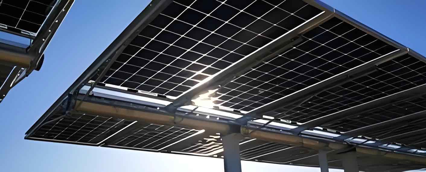
As the global energy crisis and environmental concerns intensify, renewable energy sources have become a central pillar of modern energy strategies. Among them, solar energy stands out due to its abundance, cleanliness, and sustainability. Solar panels, also known as photovoltaic panels, convert sunlight directly into electricity through the photovoltaic effect. However, during long-term outdoor operation, solar panels are exposed to harsh environmental conditions such as wind, sand, rain, temperature fluctuations, and accumulation of dust or bird droppings. These factors can lead to various surface and internal defects, including corner breakage, cracks, scratches, and hot spots. Such defects significantly reduce the power conversion efficiency of a photovoltaic system and may even cause safety hazards such as fire. Therefore, prompt and accurate detection of solar panel defects is of paramount importance for maintaining the performance and reliability of photovoltaic power stations.
Traditional defect detection methods rely heavily on manual inspection or sensor-based electrical measurement. Manual visual inspection is time-consuming, subjective, and prone to errors, especially when photovoltaic arrays are deployed in remote or large-scale installations. Sensor-based methods, such as those measuring current–voltage characteristics, require extensive wiring and periodic maintenance, which increases operational costs. To overcome these limitations, image-based detection techniques combined with deep learning have emerged as a promising solution. In particular, electroluminescence (EL) imaging provides a high-contrast visualization of internal defects in solar cells, making it an ideal modality for automatic defect detection. By applying a forward bias voltage to the panel, the radiative recombination of charge carriers generates near-infrared light, which can be captured by a CCD camera. Defective areas emit fewer photons and appear darker in the EL image, while healthy regions appear brighter. This clear contrast enables deep learning models to identify defect patterns effectively.
Deep learning-based object detection algorithms have revolutionized computer vision tasks. Two main categories exist: two-stage detectors, such as Faster R-CNN, and one-stage detectors, such as YOLO and SSD (Single Shot Multibox Detector). SSD is particularly attractive because it combines high detection accuracy with real-time processing speed. It utilizes a set of default bounding boxes over multiple feature maps of different scales and directly predicts class confidences and box offsets. Nevertheless, SSD has a known weakness in detecting small objects due to insufficient semantic information in its shallow feature layers. Additionally, the direct connection between low-level feature maps and prediction modules creates a dual learning conflict: the shallow layers must simultaneously learn detailed local features and abstract high-level semantics, which complicates training and limits accuracy.
To address these problems, my research focuses on improving the SSD architecture specifically for solar panel defect detection. I propose two major enhancements. First, I introduce a deep residual structure between the feature extraction backbone and the prediction layers. This structure separates the feature learning task from the prediction task, allowing each feature layer to be transformed into a more abstract representation before classification and regression. This alleviates the dual-learning conflict and improves detection accuracy. Second, I propose a multi-layer feature fusion method based on feature pyramids. By fusing high-level semantic features into shallow layers through transposed convolution, the shallow feature maps gain richer semantic information, leading to significantly better small defect detection performance. The entire improved model is evaluated on a public PVEL-AD dataset, and the experimental results demonstrate the effectiveness of the proposed methods.
1. Background and Significance
Photovoltaic panels are the core components of solar power generation systems. Their efficiency depends on material quality, environmental conditions, and maintenance. In practical operation, defects such as micro-cracks, scratches, corner breakage, and hot spots can develop due to mechanical stress, thermal cycling, and contamination. These defects cause local regions to absorb more sunlight or resist current flow, thereby generating heat and reducing output power. Hot spots, in particular, are dangerous; they can accelerate cell degradation and even ignite fires. Therefore, reliable defect detection is vital for the safety and economic viability of photovoltaic plants.
Traditional detection approaches can be classified into two categories:
| Category | Working Principle | Advantages | Disadvantages |
|---|---|---|---|
| Electrical signature based | Measure voltage, current, power, and environmental data | Direct electrical parameter feedback | Complex wiring, high cost, low flexibility |
| Image based | Use thermal or EL imaging to visualize defective regions | Non-contact, fast, high localization accuracy | Requires high-quality images and robust algorithms |
The electrical signature approach relies on sensors installed around the photovoltaic array. Although it can identify global faults such as short circuits or open circuits, it is difficult to pinpoint the exact location of a defect on a specific cell. Moreover, the installation and maintenance of sensors add significant labor and material costs. Image-based methods, especially EL imaging, offer a spatial resolution that allows precise localization of the defect. When combined with convolutional neural networks (CNNs), the detection process can be fully automated, eliminating the need for human expertise and enabling large-scale inspection via drones or mobile robots.
The significance of this research lies in:
- Providing a fast and accurate method to detect solar panel defects using EL images, which is crucial for maintaining power generation efficiency.
- Reducing reliance on manual inspection, thus lowering operational costs and improving safety.
- Extending the service life of photovoltaic panels by enabling timely maintenance before catastrophic failures occur.
- Demonstrating the effectiveness of deep residual structures and feature pyramid fusion for small object detection in industrial applications.
- Offering a potential framework for real-time monitoring systems in smart photovoltaic plants.
2. Fundamentals of Convolutional Neural Networks and Object Detection
2.1 Convolutional Neural Network Basics
Convolutional neural networks (CNNs) are the backbone of modern object detection. A typical CNN consists of convolution layers, pooling layers, activation functions, and fully connected layers. The convolution layer extracts features by sliding a set of learnable kernels over the input image. Each kernel computes a weighted sum of the local receptive field and produces a feature map. The convolution operation is expressed as:
$$x_j^{(n)} = \sum_i x_i^{(n-1)} * k_{ij}^{(n)} + b_j^{(n)}$$
where \(x_i^{(n-1)}\) is the input feature map, \(k_{ij}^{(n)}\) is the convolutional kernel, \(b_j^{(n)}\) is the bias term, and \(*\) denotes the convolution operator. After convolution, an activation function such as ReLU is applied to introduce nonlinearity. The ReLU activation function is defined as:
$$f(x) = \max(0, x)$$
Pooling layers downsample the feature maps, thereby reducing computational complexity and enhancing translation invariance. Common pooling operations include max pooling and average pooling. A fully connected layer at the end of the network flattens the high-level features and performs classification.
One of the key properties of CNNs is weight sharing, which significantly reduces the number of parameters. Additionally, the hierarchical structure of CNNs allows low-level layers to capture edges and colors, while deeper layers extract semantic concepts such as shapes and object parts. This hierarchy is exploited by multi-scale detection models like SSD.
2.2 Modern Object Detection Models
Object detection algorithms can be divided into two families: two-stage and one-stage. Two-stage detectors first generate region proposals and then classify each proposal. The representative architecture is Faster R-CNN, which uses a Region Proposal Network (RPN) to generate candidate boxes and then performs classification and bounding box regression. Two-stage detectors generally achieve higher accuracy but at the cost of slower inference speed. One-stage detectors, including YOLO and SSD, directly predict objects from feature maps in a single pass. They perform regression and classification simultaneously, making them much faster and more suitable for real-time applications.
SSD is an outstanding one-stage detector. It inherits the anchor mechanism from Faster R-CNN and the regression idea from YOLO. The SSD network uses a pre-trained backbone network, usually VGGNet, to extract features. Then it applies several convolutional layers of decreasing sizes to generate multi-scale feature maps. For each feature map cell, a set of default boxes with different scales and aspect ratios is generated. The network predicts the class probabilities and the offsets for each default box. The total loss is a weighted sum of localization loss and confidence loss:
$$L = \frac{1}{N}(L_{conf} + \alpha L_{loc})$$
where \(N\) is the number of matched default boxes, \(\alpha\) is the weight factor, \(L_{loc}\) is the Smooth L1 loss for box offsets, and \(L_{conf}\) is the softmax loss for class confidence.
| Detector Type | Example | Advantages | Disadvantages |
|---|---|---|---|
| Two-stage | Faster R-CNN | High accuracy | Slow inference, complex pipeline |
| One-stage | YOLO, SSD | Real-time speed | Lower accuracy for small objects |
2.3 Image Preprocessing and Augmentation for Solar Panels
Image preprocessing is essential to improve the quality of EL images and enhance the robustness of the detection algorithm. Common techniques include:
- Grayscale conversion: EL images are usually captured as grayscale or can be converted to reduce computational load. The intensity \(f(x,y)\) represents the luminance at pixel coordinates \((x,y)\).
- Geometric transformation: Corrects distortions caused by camera angles, rotation, or scale changes. This is especially useful when images are captured from drones.
- Normalization: Scales pixel values to a fixed range, which stabilizes training and accelerates convergence.
- Smoothing and filtering: Removes noise while preserving edge and defect structures.
- Image augmentation: Expands the dataset by applying random brightness changes, horizontal flips, vertical flips, affine transformations, Gaussian blur, and noise injection. Augmentation increases generalization and reduces overfitting.
For my experiments, the PVEL-AD dataset is used, which consists of 2,176 EL images of photovoltaic cells. Each image is annotated with bounding boxes for four defect types: corner breakage, cracks, scratches, and hot spots. The dataset is divided into training, validation, and testing subsets with a ratio of 6:2:2. All images are preprocessed and augmented randomly using the techniques mentioned above.
3. Deep Residual Structure for Improved SSD
3.1 Analysis of SSD Network Architecture
In the standard SSD network, a pre-trained VGGNet serves as the backbone. Features are extracted at six different layers: Conv4-3, Conv5-3, Conv6-2, Conv7-2, Conv8-2, and Conv9-2. The prediction modules, consisting of a 3×3 convolution for class confidence and another 3×3 convolution for bounding box regression, are directly attached to each of these feature maps. This design enables detection at multiple scales: smaller objects are detected from earlier layers with higher resolution, while larger objects are detected from deeper layers with lower resolution but richer semantics. However, the direct attachment creates a conflict. The shallow layers, such as Conv4-3, need to provide accurate local details for predicting small objects, but they must also pass adequate semantic information to the deeper layers through the sequential network. Learning both tasks simultaneously in the same layer increases optimization difficulty and degrades overall performance.
The mathematical formulation of the multi-scale prediction is:
$$\mathcal{P}(x) = \left\{ P_{s_1}(x_{s_1}), P_{s_2}(x_{s_2}), \dots, P_{s_k}(x_{s_k}) \right\}$$
where \(x_{s_i}\) denotes the feature map at layer \(s_i\), and \(P_{s_i}\) is the prediction function for that layer. For a shallow feature layer \(x_{s_1}\), the feature is computed as:
$$x_{s_1} = F_{s_1} \circ F_{s_1 – 1} \circ \dots \circ F_1(I)$$
where \(I\) is the input image and \(F_i\) are nonlinear transformations. The layer \(x_{s_1}\) must simultaneously minimize the prediction loss and provide useful features for subsequent layers. This undesired coupling is the fundamental problem I aim to solve.
3.2 Deep Residual Learning
Deep residual networks (ResNets) were introduced by He et al. to ease the training of very deep networks. Instead of fitting a direct mapping from input to output, a residual block learns the residual mapping. The output of a residual block is:
$$y_t = \mathcal{F}(x_t, W_t) + x_t$$
where \(x_t\) is the input to the block, \(\mathcal{F}\) represents the stacked nonlinear layers (convolution, batch normalization, ReLU), and \(W_t\) are the trainable weights. If the optimal mapping is close to identity, the residual mapping is easier to learn than the original mapping. The skip connection provides an alternative path for gradients during backpropagation, mitigating the vanishing gradient problem. In general, for a network with \(T\) consecutive residual blocks, the error gradient with respect to the input of block \(t\) is:
$$\frac{\partial \mathcal{L}}{\partial x_t} = \frac{\partial \mathcal{L}}{\partial x_T} \prod_{k=t}^{T-1} \frac{\partial}{\partial x_k} \left[ \mathcal{F}(x_k, W_k) + x_k \right]$$
Because the derivative of the skip connection is exactly 1, the product term contains a sum of identity mappings, which stabilizes gradient propagation and makes training a very deep model feasible.
For my improvement, I integrate residual blocks into the SSD architecture. Instead of directly attaching prediction layers to the original feature maps, I insert a residual block after each feature map. This block transforms the original feature map into a more abstract representation that is then used for prediction. At the same time, the original feature map still flows through the backbone to subsequent layers, preserving local details. This separation effectively resolves the dual-learning conflict.
3.3 Design of the Improved Deep Residual Structure
I design a double-branch residual module that is appended to each of the six selected feature maps in SSD. The structure is illustrated conceptually in the following block:
| Layer | Input Channels | Output Channels | Kernel Size | Stride | Padding |
|---|---|---|---|---|---|
| 1×1 Convolution | \(C_{in}\) | 128 | 1 | 1 | 0 |
| 3×3 Convolution | 128 | 128 | 3 | 1 | 1 |
| 1×1 Convolution | 128 | 256 | 1 | 1 | 0 |
| Skip connection | \(C_{in}\) | 256 | 1×1 projection if needed | – | – |
The final output of the residual module is:
$$z_t = \mathcal{R}(x_t) = \mathcal{G}(x_t, W_g) + \mathcal{H}(x_t, W_h)$$
where \(\mathcal{G}\) is the main convolutional branch and \(\mathcal{H}\) is a 1×1 convolution used to project the input to 256 channels if the channel number differs. For all six feature maps in the VGG-based SSD, the input channel numbers range from 256 to 1024. After the transformation, all residual modules output feature maps with 256 channels. This uniform channel number simplifies subsequent feature fusion and reduces computational overhead.
The benefit of using the double-branch residual structure is twofold. First, the residual connection helps gradient flow and makes the training more efficient. Second, the structure itself acts as a feature refinement module, generating more discriminant features for the prediction layers. This is particularly important for shallow layers because the refined features become more abstract while still retaining the required spatial resolution for small object localization.
4. Feature Pyramid Multi-Layer Feature Fusion
4.1 Semantic Information in Different Feature Layers
The receptive field is a crucial concept in understanding semantic information. For a given convolutional layer, the receptive field is the region of the input image that affects a single output neuron. A larger receptive field implies that the neuron encodes more global context, while a smaller receptive field indicates more local details. The receptive field size can be computed recursively:
$$r_{out} = r_{in} + (k – 1) \prod_{i=1}^{l} s_i$$
where \(r_{in}\) and \(r_{out}\) are the receptive fields before and after the convolution kernel of size \(k\), \(s_i\) is the stride of the \(i\)-th preceding layer. For the SSD network with a 300×300 input, the receptive fields of the six feature layers are summarized below:
| Feature Layer | Resolution | Receptive Field |
|---|---|---|
| Conv4-3 | 38×38 | 60 |
| Conv5-3 | 19×19 | 92 |
| Conv6-2 | 10×10 | 132 |
| Conv7-2 | 5×5 | 164 |
| Conv8-2 | 3×3 | 228 |
| Conv9-2 | 1×1 | 356 |
It is evident that small objects are mainly detected by Conv4-3 and Conv5-3, whose receptive fields are much smaller than those of deeper layers. Consequently, these shallow layers contain insufficient semantic context to distinguish confusing defects or background clutter. This is the core reason why SSD underperforms on small defect detection.
4.2 Feature Pyramid Networks and Image Pyramid
An image pyramid constructs multiple resolutions of the same image to detect objects at different scales. However, applying a convolutional network to every level of the image pyramid is computationally prohibitive. Feature Pyramid Network (FPN) proposed by Lin et al. offers a more elegant solution. FPN leverages the natural hierarchical feature pyramid of a CNN and adds top-down pathways with lateral connections. High-level semantic features are upsampled and combined with lower-level features, enhancing the semantic quality of all layers at a modest increase in computation.
For SSD, the natural multi-scale predictions already form a kind of pyramid. However, the lack of top-down fusion limits the semantic richness of shallow layers. I therefore design a feature fusion strategy that augments the first three layers (Conv4-3, Conv5-3, Conv6-2) with semantic information from deeper layers. The fusion is implemented using a three-branch structure that extends the residual module defined earlier.
4.3 Transposed Convolution for Feature Upsampling
To fuse a deep feature map with a shallower feature map, we need to match their spatial dimensions and channel counts. This is achieved using transposed convolution, also known as deconvolution. In matrix form, convolution can be represented as:
$$y = A x$$
where \(x\) is the input vector, \(y\) is the output vector, and \(A\) is the convolution matrix. Transposed convolution multiplies the loss gradient by \(A^T\) during the forward pass, effectively performing upsampling with learnable parameters. A common use is to enlarge feature maps while preserving semantic information. In my design, a deep feature map (e.g., Conv5-3) is first passed through a 3×3 convolution to reduce the channel count, then upsampled by a 2×2 transposed convolution with stride 2, and finally projected to the desired number of channels by a 1×1 convolution.
4.4 Design of Multi-Layer Feature Fusion
I propose the SSD-F3 structure, which fuses the first three feature layers (Conv4-3, Conv5-3, Conv6-2) with their immediate successors. More specifically:
- Conv4-3 is fused with the refined version of Conv5-3.
- Conv5-3 is fused with the refined version of Conv6-2.
- Conv6-2 is fused with the refined version of Conv7-2.
The refined deep feature is generated by a transformation path \(T\) consisting of a 3×3 convolution, a 2×2 transposed convolution, and a 1×1 convolution. The transformed feature is then added element-wise to the shallow feature after the residual module. This yields a three-branch structure: the original residual branch, the newly added fusion branch, and the identity skip connection. The operation can be expressed as:
$$y_{n} = \mathcal{R}(x_n) + \mathcal{U}(x_{n+1}) + x_n$$
where \(\mathcal{R}\) denotes the convolutional transformation of the shallow layer, \(\mathcal{U}\) denotes the upsampling transformation of the deeper layer, and \(x_n\) is the original feature map used as the identity branch. All branches produce tensors of identical shape (e.g., 38×38×256 for Conv4-3).
I also considered fusing all five feature layers (SSD-F5), but experiments showed that the additional computational cost grows substantially while the accuracy gain is marginal. Therefore, the SSD-F3 structure provides a better trade-off between accuracy and speed.
5. Simulation Experiments and Analysis
5.1 Experimental Setup
I built an EL detection simulation platform based on an FPGA development board with a ZYNQ-7020 core and an OV5640 image sensor. Although the final dataset used for training is the PVEL-AD dataset due to the unavailability of a professional CCD camera for field data acquisition, the platform successfully simulates the process of capturing EL images from solar panels. The platform consists of a DC power supply, a power controller, a solar cell, an imaging system, and an image processing unit. The captured images are transmitted to a host computer for further analysis.
The deep learning experiments were conducted on a computer with an Intel Core i5-10200H CPU, an NVIDIA GeForce GTX 1650 Ti GPU, Python 3.8, and PyTorch 1.7.1. The training process had 100 epochs, with a two-stage strategy: the first 50 epochs froze the backbone networks to save memory (batch size 16), and the remaining 50 epochs fine-tuned the whole network (batch size 8). The input image size was 416×416. I used a cosine annealing learning rate schedule varying between \(1 \times 10^{-4}\) and \(1 \times 10^{-2}\), and the SGD optimizer.
5.2 Dataset Preparation
The PVEL-AD dataset contains 2,176 EL images of photovoltaic cells. I selected four defect categories: corner breakage, crack, scratch, and hot spot (referred to as “Black core” in the dataset annotation). Using LabelImg software, each defect was annotated with a rectangular bounding box, and the annotations were saved in XML format following the PASCAL VOC standard. The XML files were converted into CSV files for easier data loading. To expand the training data and improve generalization, I applied augmentation methods including random brightness variation, left-right mirroring, top-bottom flipping, affine transformations, Gaussian blur, and additive noise. A Gaussian blur kernel is defined as:
$$G(x,y) = \frac{1}{2\pi \sigma^2} e^{-\frac{x^2 + y^2}{2 \sigma^2}}$$
where \(\sigma\) is the blur radius, randomly chosen from 0 to 3 in my experiments. After augmentation, the dataset size increased significantly, and the model became more robust to variations in image capturing conditions.
5.3 Simulation Experiment 1: Deep Residual SSD
In this experiment, I compared three models:
- SSD: the original SSD model without any extra structure.
- SSD-DR: SSD with the proposed deep residual structure appended to each detection layer.
- SSD-Conv: SSD with a plain convolutional block of similar capacity but without skip connections.
The results after 100 epochs are summarized in the following table:
| Model | Corner AP (%) | Crack AP (%) | Scratch AP (%) | Hot Spot AP (%) | mAP (%) | Frame Rate (FPS) |
|---|---|---|---|---|---|---|
| SSD | 89.8 | 88.1 | 82.3 | 90.2 | 87.6 | 47.3 |
| SSD-DR | 91.4 | 90.7 | 84.5 | 92.7 | 89.8 | 42.5 |
| SSD-Conv | 89.9 | 88.7 | 83.7 | 91.8 | 88.5 | 43.1 |
The results demonstrate that both modifications improve mAP over the baseline. However, SSD-DR achieves a 2.2% higher mAP than SSD, while SSD-Conv improves only by 0.9%. The reason is that the residual connection in SSD-DR facilitates gradient propagation and leads to more effective training. The frame rate of SSD-DR decreases by only 4.8 FPS relative to the original SSD, which is acceptable for practical applications. Thus, the deep residual structure effectively enhances detection accuracy without severely compromising speed.
5.4 Simulation Experiment 2: Feature Pyramid Fusion
In the second experiment, I evaluated the proposed SSD-F3 and the alternative SSD-F5 against the SSD-DR model. The comparison metrics are shown below:
| Model | Corner AP (%) | Crack AP (%) | Scratch AP (%) | Hot Spot AP (%) | mAP (%) | Frame Rate (FPS) |
|---|---|---|---|---|---|---|
| SSD | 89.8 | 88.1 | 82.3 | 90.2 | 87.6 | 47.3 |
| SSD-DR | 91.4 | 90.7 | 84.5 | 92.7 | 89.8 | 42.5 |
| SSD-F3 | 93.2 | 92.5 | 87.1 | 94.5 | 91.8 | 41.8 |
| SSD-F5 | 93.4 | 93.1 | 86.6 | 94.9 | 92.0 | 38.7 |
SSD-F3 improves mAP by 2.0% over SSD-DR, reaching 91.8%. The improvement is especially notable for the scratch class, which is typically small and difficult to detect. SSD-F5 achieves a slightly higher mAP (92.0%) but at the expense of a much lower frame rate (38.7 FPS). The 3.1 FPS reduction from SSD-F3 to SSD-F5 is disproportionate to the small accuracy gain. Therefore, SSD-F3 is chosen as the optimal trade-off between accuracy and speed.
To further verify the effectiveness of SSD-F3 on small defects, I split the test samples into three scales: small, medium, and large. The average precision for each scale is reported below:
| Model | Test Sample Scale | mAP (%) |
|---|---|---|
| SSD | Small | 82.6 |
| SSD-F3 | Small | 87.4 |
| SSD | Medium | 89.6 |
| SSD-F3 | Medium | 92.5 |
| SSD | Large | 90.2 |
| SSD-F3 | Large | 93.9 |
The improvement for small scale targets is 5.8 percentage points, which is the highest among all scales. This clearly confirms the advantage of the feature pyramid fusion method in enhancing shallow semantic information and improving small defect detection.
5.5 Visualization and Loss Analysis
During training, I monitored the loss function curves. The loss decreased smoothly and converged after about 100 epochs, showing the stability of the improved architecture. The training loss is composed of localization loss and confidence loss. The combined loss function for the entire model is given by:
$$\mathcal{L} = \frac{1}{N} \left( \mathcal{L}_{conf} + \alpha \mathcal{L}_{loc} \right)$$
where \(\alpha\) is set to 1 in my experiments. The smooth convergence proves that the residual connections and feature fusion layers do not introduce instability.
I also compared the actual detection outputs on several test images. The original SSD often misses small cracks and scratches, while the improved SSD-F3 successfully detects them with high confidence. The visual comparisons highlight that the proposed model better captures the subtle intensity variations characteristic of photovoltaic cell defects.
6. Conclusion and Future Work
In this paper, I presented an improved SSD algorithm for detecting surface defects in solar panels using EL images. The main contributions are as follows.
First, I analyzed the dual-learning conflict in the standard SSD architecture, where shallow feature layers are responsible for both local detail extraction and high-level semantic abstraction. To solve this problem, I introduced a deep residual structure between the backbone and the prediction layers. This structure enables each feature map to be refined into a more abstract representation before being used for object detection. Experimental results show that the SSD-DR model achieves a 2.2% mAP improvement over the baseline with a small reduction in frame rate.
Second, I designed a multi-layer feature fusion mechanism based on feature pyramids. By using transposed convolution to upsample deep feature maps and then adding them to shallow feature maps, the semantic information of the shallow layers is significantly enhanced. The resulting SSD-F3 model further improves mAP by 2.0% over SSD-DR and, more importantly, achieves a 5.8% improvement on small-scale defect detection. This confirms that the feature fusion method effectively boosts the performance of detecting small defects such as scratches and cracks.
Third, I built an FPGA-based EL simulation platform to mimic the real inspection process. Although the experiments were carried out on the public PVEL-AD dataset, the complete pipeline demonstrates the feasibility of automated solar panel inspection using drone-mounted imaging devices.
There is still room for improvement. The current network runs at about 42 FPS, which is real-time but could be further optimized. In future work, I plan to incorporate pruning techniques to reduce model complexity and increase inference speed. Additionally, I will explore more advanced backbone networks such as ResNet or EfficientNet to improve feature extraction quality. More diverse and larger EL datasets are also needed to make the model more robust in real-world scenarios. Finally, the proposed method could be extended to other photovoltaic defect types, such as finger interruption and soldering defects, which are also observable in EL images.
In summary, the proposed improved SSD algorithm, combining deep residual structures and feature pyramid fusion, is an effective solution for solar panel defect detection. It achieves high accuracy and real-time speed, making it suitable for practical deployment in photovoltaic power stations and contributing to the safe and efficient operation of solar energy systems.