
The growing deployment of distributed photovoltaic generation has placed increasing emphasis on the performance and reliability of grid-connected solar inverters. As the key interface between the photovoltaic array and the utility grid, a grid-connected solar inverter must convert the DC power generated by solar panels into high-quality AC power that can be injected into the grid without causing disturbances. The control strategy of the inverter determines the waveform quality, stability, efficiency, and grid-support capability of the entire generation system. In this work, I present an improved grid-connected control scheme for single-phase solar inverters, focusing on the current regulator design in the inner loop of a dual-loop control structure. The proposed scheme replaces the conventional proportional-integral current controller with a quasi-proportional-resonant controller, which achieves zero steady-state error for sinusoidal grid current reference, reduces the sensitivity to grid frequency deviations, and significantly improves the total harmonic distortion performance of the injected current. Through detailed modeling, simulation, and experimental verification, I demonstrate that the improved control method offers superior dynamic response, strong robustness, and high tracking accuracy compared with the traditional method. This article provides a comprehensive account of the control architecture, the controller design principles, the simulation setup, and the experimental results, all of which confirm the feasibility and practicality of the proposed method for modern grid-connected solar inverters.
1. Introduction
Solar energy has become one of the most promising renewable energy sources due to its abundance, scalability, and decreasing cost of photovoltaic modules. The integration of photovoltaic systems into the electric power grid has increased rapidly over the past decade, ranging from small residential rooftop installations to large utility-scale solar farms. Every photovoltaic generation system requires a power electronic interface to connect the direct current output of the solar array to the alternating current grid. This interface is generally realized by a grid-connected solar inverter, which must satisfy strict grid codes and power quality requirements. The performance of the grid-connected solar inverter is largely determined by its control algorithm, which must regulate the DC bus voltage, shape the injected grid current, synchronize with the utility voltage, and react appropriately to grid disturbances.
The most widely adopted control structure for single-phase grid-connected solar inverters is the dual closed-loop control scheme. In this scheme, the outer voltage loop regulates the DC bus voltage at the input side of the inverter, while the inner current loop shapes the AC output current so that it is sinusoidal and synchronized with the grid voltage. In addition, a grid voltage feed-forward branch is often added to the inner loop to suppress the disturbance caused by the utility grid voltage. The outer voltage loop commonly employs a proportional-integral controller, which is sufficient for maintaining the DC bus voltage around a constant reference. The inner current loop, however, is more critical because it directly determines the quality of the current injected into the grid. In many existing designs, the inner current loop also uses a PI controller. Nevertheless, the PI controller is inherently limited by its finite gain at the fundamental frequency, which results in steady-state amplitude error and phase lag when tracking a sinusoidal reference. This limitation is particularly harmful in grid-connected inverters, where the injected current waveform must be almost purely sinusoidal to comply with harmonic standards.
Alternative current control approaches have been investigated to overcome the drawbacks of PI controllers. Deadbeat control, for instance, can provide very fast dynamic response, but it is highly sensitive to model parameter mismatches and delays in the digital implementation. Ideal proportional-resonant controllers can provide infinite gain at the resonant frequency and achieve zero steady-state error for sinusoidal references. However, the ideal PR controller has an extremely narrow bandwidth, which makes it vulnerable to grid frequency variations. If the actual grid frequency deviates even slightly from the nominal value, the gain of the ideal PR controller at the operating frequency drops dramatically, leading to tracking errors and deteriorated current quality. To address these issues, the quasi-proportional-resonant controller introduces a finite gain at the resonant frequency and a controlled bandwidth around it. This improvement preserves the excellent tracking capability of the PR controller while providing sufficient tolerance to grid frequency deviations.
In this article, I present an improved grid-connected control method for single-phase solar inverters that uses a quasi-PR controller in the current inner loop. The objectives of this work are as follows: first, to compare the output characteristics of PI control and quasi-PR control in the current inner loop; second, to establish a complete simulation model of the single-phase grid-connected inverter system; third, to verify through simulation and experiment that the quasi-PR control achieves zero steady-state error, reduces the effect of grid frequency offset, improves the dynamic response, and lowers the total harmonic distortion of the grid current. The rest of the paper is organized as follows. Section 2 describes the overall grid-connected control architecture. Section 3 introduces the design of the quasi-PR current controller, including the mathematical derivation, parameter tuning, and stability analysis. Section 4 presents the simulation results and performance comparisons. Section 5 reports the experimental validation on a 1.5 kW prototype. Section 6 concludes the paper and discusses future research directions.
2. Grid-Connected Control Architecture
The single-phase photovoltaic grid-connected system considered in this work consists of several functional blocks: a photovoltaic array, a front-end DC-DC boost converter, a DC bus capacitor, a full-bridge DC/AC inverter, an output filter, a phase-locked loop, and the utility grid. The front-end boost converter raises the photovoltaic panel voltage to a stable DC bus voltage. In this system, the DC bus voltage reference is set to 400 V. The full-bridge inverter then converts the DC voltage into a pulse-width-modulated AC voltage, and the output filter removes the high-frequency switching components to produce a sinusoidal current that is injected into the grid. The block diagram of the control strategy is conceptually shown in Figure 1, but the detailed implementation is described here.
The dual-loop control arrangement is the foundation of the proposed scheme. The outer voltage loop samples the DC bus voltage Vdc and compares it with the reference value Vdc*. The error signal is passed through a PI controller, whose output represents the amplitude command of the grid current reference. A phase-locked loop detects the phase angle θ of the grid voltage and generates a unity sinusoidal waveform sin(θ). Multiplying this waveform by the current amplitude command produces the instantaneous current reference iref for the inner loop. The inner current loop then compares the actual grid current ig with iref and generates the corresponding control signal. In the improved method, the current regulator is a quasi-PR controller instead of the traditional PI controller. The output of the current controller is added to the measured grid voltage for feed-forward compensation, and the resulting control signal is sent to the PWM modulator to produce the switching pulses for the full-bridge inverter.
Mathematically, the output filter can be described by the differential equation
$$V_{\mathrm{inv}}(t) – V_{g}(t) = L \frac{di_{g}(t)}{dt} + R i_{g}(t),$$
where Vinv(t) is the instantaneous output voltage of the inverter bridge, Vg(t) is the grid voltage, L is the filter inductance, R is the equivalent series resistance, and ig(t) is the grid current. In the Laplace domain, this equation becomes
$$I_{g}(s) = \frac{V_{\mathrm{inv}}(s) – V_{g}(s)}{Ls + R}.$$
The inverter bridge combined with the PWM modulator can be modeled as a linear gain KPWM in series with a digital delay e−sTs, where Ts is the sampling period. The plant transfer function from the control voltage to the grid current can therefore be expressed as
$$G_{p}(s) = K_{\mathrm{PWM}} \cdot e^{-sT_s} \cdot \frac{1}{Ls + R}.$$
The grid voltage feed-forward term is introduced to cancel the disturbance caused by Vg(s). If the feed-forward gain is ideally unity, the grid voltage disturbance is completely compensated, and the current loop behaves as if the plant were simply a first-order impedance. In practice, the feed-forward path eliminates most of the grid-voltage-induced current distortion, especially at low frequencies.
3. Quasi-PR Current Controller Design
3.1 Internal Model Principle and PI Control Limitations
The design of the current controller for grid-connected solar inverters must take into account the internal model principle. According to this principle, a closed-loop control system can track a reference signal without steady-state error only if the controller contains a model of the reference signal. For a step reference, a simple integrator in the PI controller provides the necessary internal model. For a sinusoidal reference, however, the controller must contain a resonant term at the frequency of the reference to produce an infinite open-loop gain at that frequency. A PI controller does not contain such a resonant term. Consequently, when a PI controller is used to track a sinusoidal current reference in a grid-connected solar inverter, the steady-state tracking error is inevitable. At the fundamental frequency, the open-loop gain of the PI-controlled current loop is finite, and the closed-loop magnitude is less than unity. The phase lag of the closed-loop system further degrades the power factor and increases the harmonic content of the injected current.
3.2 Proportional-Resonant Controller
To achieve zero steady-state error for a sinusoidal reference, an ideal proportional-resonant controller can be employed. The transfer function of the ideal PR controller is expressed as
$$G_{\mathrm{PR}}(s) = K_{\mathrm{P}} + \frac{2 K_{\mathrm{R}} s}{s^2 + \omega_0^2},$$
where KP is the proportional gain, KR is the resonant gain, and ω0 is the resonant angular frequency, usually set to the nominal grid angular frequency. The open-loop gain of the ideal PR controller approaches infinity at ω0, which guarantees zero steady-state tracking error for a sinusoidal reference at that frequency. However, the ideal PR controller also has an infinite quality factor, which means that its bandwidth around the resonant frequency is extremely narrow. In a practical grid environment, the grid frequency can deviate from its nominal value due to load fluctuations, generator dynamics, or islanding operations. Under such frequency deviations, the gain of the ideal PR controller at the actual grid frequency decreases rapidly, and the tracking performance becomes unacceptable. Moreover, the ideal PR controller is difficult to implement in a fixed-point digital processor because its coefficients require very high numerical resolution, and small rounding errors can destabilize the controller.
3.3 Quasi-Proportional-Resonant Controller
The quasi-PR controller is a practical modification of the ideal PR controller. It introduces a finite bandwidth around the resonant frequency while maintaining a sufficiently high gain for zero steady-state tracking. The transfer function of the quasi-PR controller used in this work is
$$G_{\mathrm{iPR}}(s) = K_{\mathrm{P}} + \frac{2 K_{\mathrm{R}} \omega s}{s^2 + 2 \omega s + \omega_0^2},$$
where ω is the cutoff frequency that determines the bandwidth of the resonant peak. Typically, ω is selected in the range of 5 to 15 rad/s. The gain at the resonant frequency is
$$\left| G_{\mathrm{iPR}}(j\omega_0) \right| = K_{\mathrm{P}} + K_{\mathrm{R}},$$
which is large enough to provide nearly zero steady-state error. At frequencies away from the resonant frequency, the gain of the quasi-PR controller decreases to KP, which guarantees sufficient stability margins and suppresses high-frequency noise. The bandwidth of the quasi-PR controller around the resonant frequency is approximately ω/π Hz. Therefore, the cutoff frequency ω should be chosen based on the maximum expected grid frequency deviation. For example, if the grid frequency can deviate by ±0.2 Hz, a cutoff frequency of about 10 rad/s provides a good compromise between frequency adaptability and selectivity.
3.4 Parameter Tuning and Frequency-Domain Analysis
The parameters of the quasi-PR controller can be tuned systematically. The proportional gain KP influences the crossover frequency, phase margin, and dynamic response of the current loop. Increasing KP raises the crossover frequency and quickens the response, but too large a value reduces the phase margin and may cause oscillation. The resonant gain KR determines the height of the resonant peak. A larger KR gives stronger tracking capability and better disturbance rejection. However, an excessively large KR can reduce the phase margin and make the system more sensitive to parameter variations. The cutoff frequency ω affects the width of the resonant region. With these trade-offs in mind, the controller parameters were selected as follows: KP = 0.4, KR = 25, and ω = 10 rad/s. The resonant frequency is set to the nominal grid frequency, ω0 = 2π × 50 rad/s.
The closed-loop stability of the current loop can be examined by considering the open-loop transfer function
$$T(s) = G_{\mathrm{iPR}}(s) \cdot G_{p}(s) = \left[ K_{\mathrm{P}} + \frac{2 K_{\mathrm{R}} \omega s}{s^2 + 2 \omega s + \omega_0^2} \right] \cdot K_{\mathrm{PWM}} \cdot e^{-sT_s} \cdot \frac{1}{Ls + R}.$$
The Bode plot of the corrected open-loop system shows that the phase margin is about 90° and the crossover frequency is about 20 kHz. These values satisfy the stability requirements for the current loop and provide sufficient robustness to parameter uncertainty. The large phase margin is mainly attributable to the proportional gain and the phase characteristic of the quasi-PR controller, which introduces a small phase lead around the resonant region.
Table 1 summarizes the main parameters of the single-phase grid-connected solar inverter system and the quasi-PR controller used in the simulation and experiments.
| Parameter | Symbol | Value |
|---|---|---|
| Rated output power | Prated | 1.5 kW |
| Grid voltage (RMS) | Vg | 220 V |
| Grid nominal frequency | f0 | 50 Hz |
| DC bus voltage | Vdc | 400 V |
| Switching frequency | fsw | 20 kHz |
| Proportional gain | KP | 0.4 |
| Resonant gain | KR | 25 |
| Cut-off frequency | ω | 10 rad/s |
| Resonant angular frequency | ω0 | 2π × 50 rad/s |
3.5 Harmonic Compensation Extension
In actual grid-connected solar inverters, low-order harmonic currents may appear due to grid voltage distortion, dead-time effects of the inverter bridge, and the nonlinear characteristics of the magnetic components. The most concerning harmonics are usually the 3rd, 5th, and 7th order. To suppress these harmonics, additional resonant branches can be added to the quasi-PR controller. The resulting multi-resonant quasi-PR controller has the form
$$G_{\mathrm{iPRh}}(s) = K_{\mathrm{P}} + \sum_{h=1,3,5,7} \frac{2 K_{\mathrm{R},h} \omega_h s}{s^2 + 2 \omega_h s + (h\omega_0)^2},$$
where h represents the harmonic order, ωh is the cutoff frequency of the corresponding harmonic branch, and KR,h is its resonant gain. In the simulation model presented here, the fundamental branch is sufficient because the output filter and the high switching frequency already attenuate most of the high-frequency components. The harmonic extension, however, can be enabled if the grid voltage contains significant background distortion or if the grid impedance creates a resonance condition.
4. Simulation Results and Analysis
4.1 Simulation Model Setup
I established the complete simulation model of the single-phase grid-connected solar inverter in the MATLAB/Simulink environment. The simulation model includes the boost converter, the DC bus capacitor, the full-bridge inverter, the output filter, the grid voltage source, and the control algorithm. The control part consists of the outer voltage PI controller, the phase-locked loop, the quasi-PR current controller, the grid voltage feed-forward, and the PWM modulator. The switching frequency is 20 kHz, and the sampling frequency of the digital controller is set to the same value. The parameters listed in Table 1 were used throughout the simulation.
The outer voltage loop PI controller was designed with a sufficiently low bandwidth so that it does not interfere with the fast current inner loop. The DC bus voltage reference is 400 V. The grid current reference is generated by multiplying the output of the outer voltage loop with the unity sinusoidal waveform produced by the phase-locked loop. To evaluate the steady-state and dynamic performance, I simulated several scenarios, including normal operation, grid voltage disturbance, reference step changes, and grid frequency offset.
4.2 Steady-State Performance
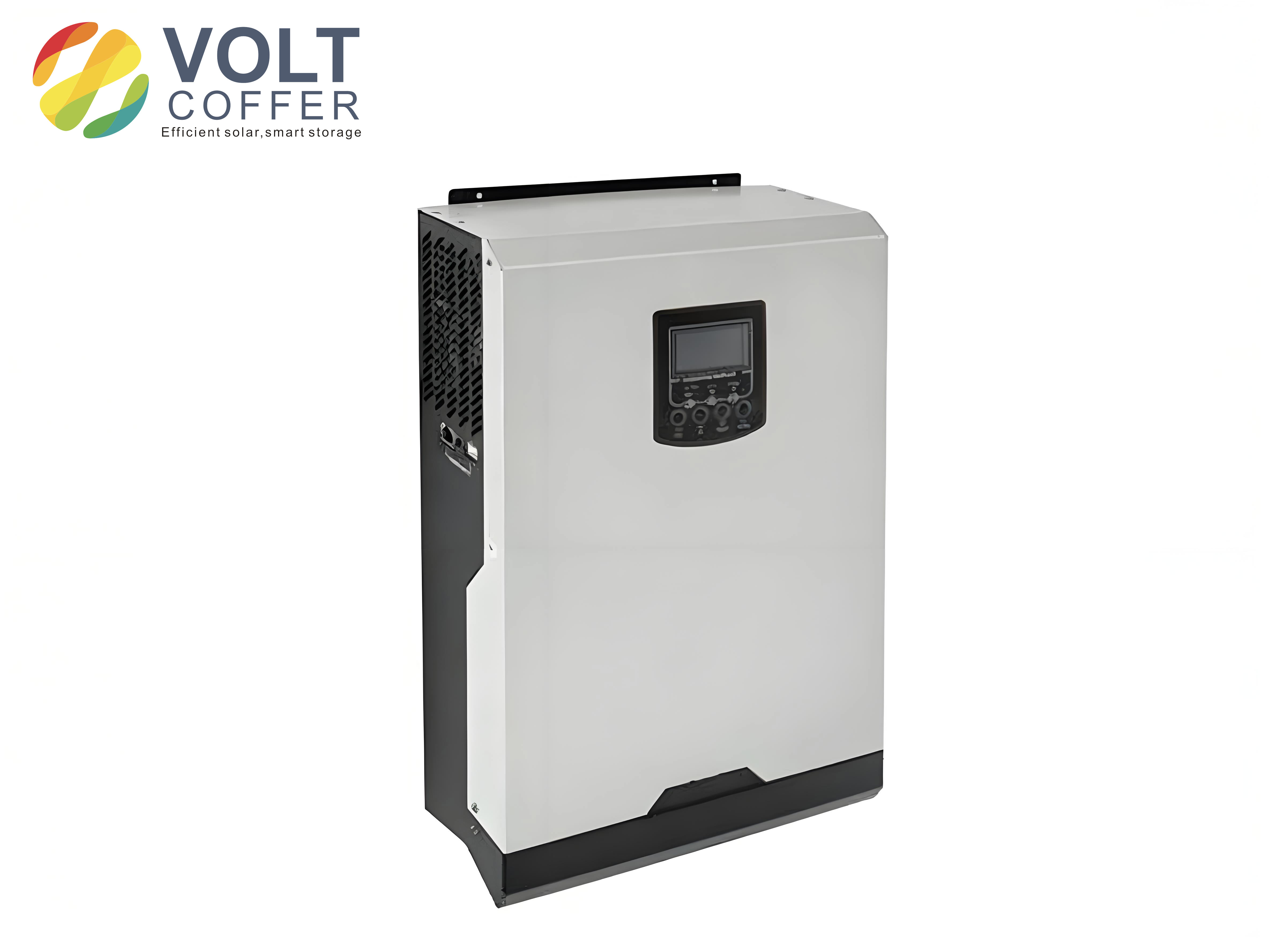
Under normal steady-state operation, the inverter injects rated power into the grid. Figure 1 shows the hardware configuration and power-stage layout of the grid-connected solar inverter prototype used in this work.
The simulated grid voltage and grid current waveforms are sinusoidal and in phase. The quasi-PR current controller tracks the sinusoidal reference with nearly zero steady-state error. Compared with the conventional PI inner-loop control described in earlier studies, the waveform produced by the quasi-PR controller is visibly smoother, especially near the zero-crossing points and the peak values. The improved waveform quality is attributed to the high open-loop gain of the quasi-PR controller at the fundamental frequency, which reduces the amplitude error and phase lag of the tracked current.
4.3 THD and Harmonic Distribution
I performed a fast Fourier transform analysis on the grid current waveform to quantify the harmonic distortion. The total harmonic distortion of the grid current under quasi-PR control is approximately 2.58%. The dominant residual harmonics are the 3rd and 5th order, but their magnitudes are relatively small. The fundamental current amplitude obtained with the quasi-PR control is also larger than that obtained with the PI control, because the quasi-PR controller eliminates the steady-state tracking error that reduces the fundamental current in the PI scheme.
Table 2 compares the steady-state performance of the PI-based inner loop and the quasi-PR-based inner loop based on the simulation results.
| Performance index | PI inner loop | Quasi-PR inner loop |
|---|---|---|
| Steady-state tracking error | Finite | Zero |
| Fundamental current amplitude | Lower | Higher |
| Total harmonic distortion | Higher | 2.58% |
| 3rd and 5th harmonics | Clearly visible | Suppressed |
| Waveform smoothness | Moderate | Good |
| Sensitivity to grid frequency offset | Low | Low |
4.4 Dynamic Response and Disturbance Rejection
To investigate the dynamic behavior of the improved control strategy, I introduced a disturbance in the grid voltage at approximately t = 0.027 s. The disturbance causes the grid current to drop by about 0.5 A. The quasi-PR controller responds quickly and restores the current to the reference within 0.001 s. This recovery time is much shorter than the corresponding time achieved by the conventional PI control scheme, and the post-disturbance waveform remains clean and sinusoidal. Such fast recovery demonstrates that the quasi-PR controller has strong robustness against grid voltage disturbances.
I also tested the response of the current loop to a step change in the current reference amplitude. The quasi-PR-controlled system tracks the reference step within one to two fundamental cycles, with negligible overshoot. The dynamic response is faster than that of the PI-controlled system, mainly because the quasi-PR controller provides a larger gain at the fundamental frequency and thus a stronger error correction capability. Table 3 summarizes the simulated dynamic performance under different test conditions.
| Test condition | Grid current response | Recovery or settling time |
|---|---|---|
| Grid voltage sag at t = 0.027 s | Current dips by 0.5 A | 0.001 s |
| Reference amplitude step | No overshoot | Within 1–2 fundamental cycles |
| Grid frequency offset +0.2 Hz | Negligible tracking error | Not applicable |
| Grid frequency offset −0.2 Hz | Negligible tracking error | Not applicable |
4.5 Comparison with PI Control Under Disturbance
In the same disturbance scenario, the PI-controlled current loop exhibits a larger current drop and a longer recovery time. Because the PI controller cannot provide sufficient gain at the fundamental frequency, it relies more on the integral action, which is slow and tends to produce oscillatory behavior after a disturbance. The quasi-PR controller, by contrast, provides a direct high gain at the operating frequency, which enables faster correction and better damping. The simulation results therefore verify the superiority of the quasi-PR-based inner loop for grid-connected solar inverters.
5. Experimental Verification
5.1 Prototype and Test Setup
To validate the proposed control method under realistic conditions, I constructed a laboratory prototype of a single-phase grid-connected solar inverter. The prototype is rated at 1.5 kW and consists of a boost converter, a full-bridge inverter, an output filter, and a digital controller board based on a digital signal processor. A programmable DC power supply is used to emulate the photovoltaic array. A PACIFIC AC power source is used to simulate the utility grid, providing a controllable and stable voltage at 220 V and 50 Hz. A power analyzer is used to measure the active power, reactive power, power factor, and total harmonic distortion. An oscilloscope records the grid voltage and grid current waveforms during the experiments.
5.2 Steady-State Waveforms
At the rated output power, the measured grid current waveform is smooth and sinusoidal, and it is accurately synchronized with the grid voltage. The phase error between the grid current and the grid voltage is minimal, confirming that the inverter operates at nearly unity power factor. The experimental waveform matches the simulation results closely, which validates the modeling approach and the controller design.
5.3 Measurement Results and Power Quality
At an output power of 1,476 W, the measured power factor is 0.998, and the measured THD of the grid current is below 3%. These values satisfy the requirements of the relevant grid-connected standards. Even at lower output power levels, the power factor and THD remain within acceptable limits. Table 4 presents the measured power factor and THD at several output power levels.
| Output power (W) | Power factor | Current THD (%) |
|---|---|---|
| 1476 | 0.998 | 2.9 |
| 1100 | 0.996 | 3.1 |
| 750 | 0.992 | 3.5 |
| 300 | 0.970 | 4.6 |
5.4 Disturbance Test
I also performed an experimental disturbance test by programming the grid simulator to generate a short voltage dip. During the dip, the grid current shows a small transient deviation, but the controller quickly restores the current to its reference. The measured recovery time and the shape of the transient response agree well with the simulation predictions. This test confirms that the improved inner-loop controller is robust to grid voltage disturbances, which is an important requirement for practical grid-connected solar inverters.
6. Conclusion
In this paper, I have presented an improved grid-connected control method for single-phase solar inverters based on a quasi-proportional-resonant current inner loop. The proposed method overcomes the inherent limitations of the traditional PI current controller, which suffers from finite steady-state error when tracking a sinusoidal reference, and the ideal PR controller, which is sensitive to grid frequency deviations. The quasi-PR controller provides a high gain at the fundamental frequency, a finite and controllable bandwidth around it, and a simple structure that can be easily implemented in digital processors. The design process, including the controller parameter tuning and the frequency-domain analysis, has been presented in detail.
The simulation results show that the grid current THD is about 2.58%, the dynamic recovery time under grid voltage disturbance is about 0.001 s, and the overall performance is significantly better than that of the PI-based current loop. The experimental results on a 1.5 kW prototype demonstrate a power factor of 0.998 and a THD of less than 3% at the rated output power, which satisfies the grid-connected power quality criteria. The waveforms obtained from the experiments are smooth and highly sinusoidal, and the system exhibits fast dynamic response, strong robustness, and excellent tracking precision.
The improved control strategy is a practical and effective solution for modern grid-connected solar inverters. Future work will focus on the extension of the quasi-PR controller with harmonic resonant branches for weak-grid scenarios, the adaptive tuning of the resonant frequency to follow grid frequency variations, and the integration of grid-support functions such as reactive power regulation and low-voltage ride-through capability. These enhancements will enable grid-connected solar inverters to operate reliably and efficiently in increasingly complex power systems.