
In the global strategic context of carbon peak and carbon neutrality, the green transformation of the transportation sector is imperative. Electric vehicles (EVs), as a cleaner, low-carbon alternative to traditional internal combustion engine vehicles, are crucial for reducing greenhouse gas emissions. This trend demands higher performance from key EV components, particularly lithium-ion batteries. Among these, Lithium Iron Phosphate (LiFePO4 or LFP) batteries have gained significant market share due to their excellent cost-effectiveness, long cycle life, and superior safety. However, effectively utilizing LFP batteries presents a core challenge for Battery Management Systems (BMS): achieving high-precision, real-time estimation of the State of Charge (SOC).
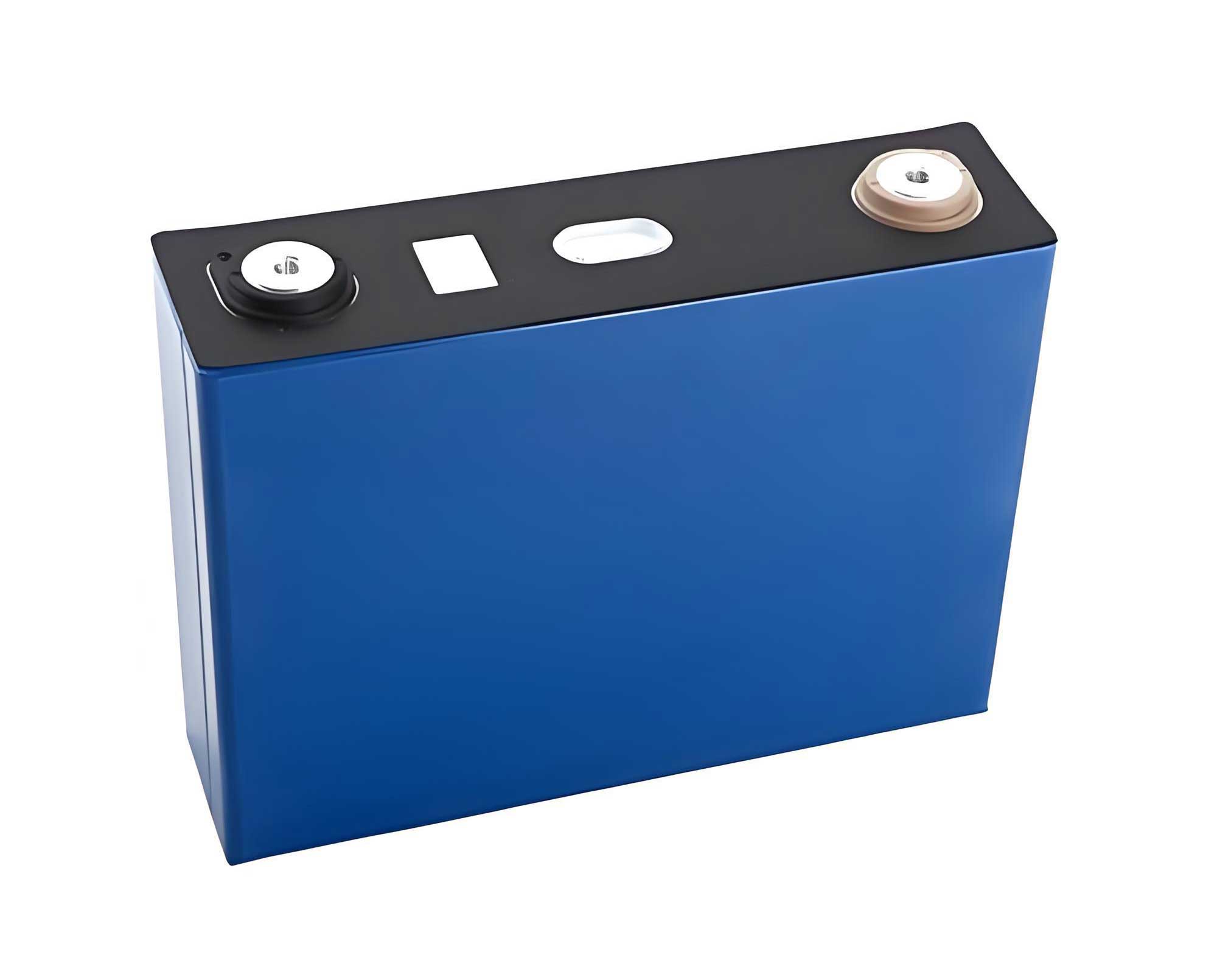
The intrinsic property of the LiFePO4 battery that complicates SOC estimation is its extremely flat Open-Circuit Voltage (OCV) versus SOC curve over a wide middle range. In this “voltage plateau,” the terminal voltage shows minimal change despite significant variations in stored energy, rendering traditional voltage-based estimation algorithms like the Extended Kalman Filter (EKF) ineffective. To overcome this material limitation, the industry has innovated at the system architecture level by proposing hybrid battery packs, where LFP cells are connected in series with Nickel Cobalt Manganese (NCM) oxide cells. The NCM chemistry exhibits a much steeper OCV-SOC relationship. This architecture cleverly uses the NCM battery’s sensitive voltage response as a dynamic reference to “calibrate” the SOC of the LFP battery during its problematic plateau region.
While this hybrid system offers a promising hardware solution, developing a robust and accurate software algorithm for SOC estimation within it remains an open research question. Simple switching between algorithms for different SOC regions often leads to discontinuous jumps in the estimated SOC value. To address these challenges, we propose a novel segmented fusion strategy for SOC estimation of LiFePO4 batteries in hybrid packs. Our method intelligently divides the operational range based on the real-time OCV slope, applies the most suitable algorithm for each segment, and ensures a smooth transition between them.
1. System Modeling and Parameter Identification
Accurate modeling is the foundation for model-based SOC estimation. We employ the first-order RC equivalent circuit model (Thevenin model) for its balance between accuracy and computational simplicity, suitable for real-time BMS applications. The model consists of an ideal voltage source (representing the OCV, $U_{oc}$), an ohmic resistor ($R_0$), and a parallel RC network ($R_1$, $C_1$) representing polarization effects.
The discrete-time state-space representation of the model is derived for implementation. The state variable is chosen as the SOC and the polarization voltage $U_1$. The system equation and measurement equation are as follows:
State Equation (Process Model):
$$ SOC_k = SOC_{k-1} – \frac{\eta \Delta t}{C_n} I_{k-1} + w_{1,k} $$
$$ U_{1,k} = \exp\left(-\frac{\Delta t}{\tau}\right) U_{1,k-1} + R_1 \left(1 – \exp\left(-\frac{\Delta t}{\tau}\right)\right) I_{k-1} + w_{2,k} $$
where $\tau = R_1 C_1$ is the time constant, $\eta$ is coulombic efficiency, $C_n$ is the nominal capacity, $\Delta t$ is the sampling interval, and $w_k$ is the process noise.
Measurement Equation (Observation Model):
$$ U_{t,k} = U_{oc}(SOC_k) – I_k R_0 – U_{1,k} + v_k $$
where $v_k$ is the measurement noise. The highly nonlinear function $U_{oc}(SOC_k)$ is the core challenge for the LiFePO4 battery.
To track the time-varying parameters of the LiFePO4 battery model (especially $U_{oc}$) online, we employ the Forgetting Factor Recursive Least Squares (FFRLS) algorithm. The terminal voltage can be expressed in a linear-in-parameters form:
$$ U_{t,k} = (1 – c_1)U_{oc,k} + c_1 U_{t,k-1} + c_2 I_k + c_3 I_{k-1} = \boldsymbol{f}_k^T \boldsymbol{\theta}_k $$
where $\boldsymbol{f}_k = [1, U_{t,k-1}, I_k, I_{k-1}]^T$ is the regressor vector and $\boldsymbol{\theta}_k = [\theta_1, \theta_2, \theta_3, \theta_4]^T$ is the parameter vector to be identified. The FFRLS algorithm updates these parameters recursively, giving more weight to recent data. The model parameters ($R_0$, $R_1$, $C_1$, $U_{oc}$) are then extracted from $\boldsymbol{\theta}_k$. The algorithm steps are summarized below:
| FFRLS Step | Calculation |
|---|---|
| 1. Gain Matrix | $ \boldsymbol{K}_k = \frac{\boldsymbol{P}_{k-1} \boldsymbol{f}_k}{\lambda + \boldsymbol{f}_k^T \boldsymbol{P}_{k-1} \boldsymbol{f}_k} $ |
| 2. Parameter Update | $ \hat{\boldsymbol{\theta}}_k = \hat{\boldsymbol{\theta}}_{k-1} + \boldsymbol{K}_k (U_{t,k} – \boldsymbol{f}_k^T \hat{\boldsymbol{\theta}}_{k-1}) $ |
| 3. Covariance Update | $ \boldsymbol{P}_k = \lambda^{-1} (\boldsymbol{I} – \boldsymbol{K}_k \boldsymbol{f}_k^T) \boldsymbol{P}_{k-1} $ |
| 4. Parameter Extraction | $ U_{oc} = \frac{\theta_1}{1 – \theta_2}, \quad R_0 = \frac{\theta_3 + \theta_2 \theta_4}{1 – \theta_2^2}, \quad R_1 = \frac{\theta_3 – \theta_4}{1 – \theta_2} – R_0, \quad C_1 = \frac{\Delta t (1 + \theta_2)}{R_1 (1 – \theta_2)} $ |
Where $\lambda$ is the forgetting factor (typically 0.95-0.999). This online identification provides a real-time estimate of the OCV, which is critical for the subsequent steps in our strategy for the LiFePO4 battery.
2. Proposed SOC Estimation Framework
The core idea of our method is to segment the discharge/charge process of the LiFePO4 battery based on the instantaneous OCV slope and to apply a dedicated, optimal estimation strategy for each segment. A smooth fusion mechanism bridges the transitions between segments to avoid SOC jumps. The overall flowchart of the proposed methodology is as follows.
2.1 OCV-Based Adaptive Slope Segmentation
The raw OCV identified online is noisy. Directly calculating its slope leads to unstable segmentation. We first apply a novel piecewise smoothing strategy tailored for the LiFePO4 battery OCV curve. In high-slope regions (beginning and end of discharge), a Savitzky-Golay filter preserves sharp features. In the middle plateau region, a moving average filter strongly suppresses noise. A sigmoid-based blending function creates smooth transitions between these two filtering zones.
Let $y_{sg}(t)$ be the Savitzky-Golay output and $y_{ma}(t)$ be the moving average output. The final smoothed OCV $S(t)$ is:
$$ S(t) = \begin{cases}
y_{sg}(t) & t \leq t_1 – \delta/2 \\
[1 – \alpha(t)]y_{sg}(t) + \alpha(t)y_{ma}(t) & t_1 – \delta/2 < t \leq t_1 + \delta/2 \\
y_{ma}(t) & t_1 + \delta/2 < t \leq t_2 – \delta/2 \\
[1 – \beta(t)]y_{ma}(t) + \beta(t)y_{sg}(t) & t_2 – \delta/2 < t \leq t_2 + \delta/2 \\
y_{sg}(t) & t > t_2 + \delta/2
\end{cases} $$
where $\alpha(t)$ and $\beta(t)$ are sigmoid transition functions centered at transition points $t_1$ and $t_2$ with width $\delta$.
We then calculate the first-order difference (slope) of $S(t)$:
$$ \text{slope}(k) = \frac{S(k) – S(k-1)}{\Delta t} $$
An adaptive threshold $Th_{slope}$ is set, typically as the maximum slope value found within the preliminarily identified plateau region. The segmentation points $p_1$ and $p_2$ are located where the slope first exceeds $Th_{slope}$ when searching backward from the plateau center and forward from the plateau center, respectively. This yields three operational zones for the LiFePO4 battery: Zone A (High SOC, High Slope), Zone B (Mid SOC, Plateau), and Zone C (Low SOC, High Slope).
2.2 Segment-Specific SOC Estimation Algorithms
For Zone A & C (High Slope): Improved Adaptive Extended Kalman Filter (AEKF)
In regions where the OCV of the LiFePO4 battery is sensitive to SOC changes, a model-based filter excels. We enhance the standard AEKF by introducing an innovation-norm-based adaptive weighting factor $\alpha_k$ to dynamically control the update strength of noise covariance matrices.
The weighting factor is computed as:
$$ \alpha_k = \alpha_{\min} + (\alpha_{\max} – \alpha_{\min}) \frac{||\boldsymbol{e}_k||^2}{||\boldsymbol{e}_k||^2 + \sigma_k} $$
where $\boldsymbol{e}_k$ is the innovation vector, and $\sigma_k$ is a running average of past innovation norms. This allows for conservative updates when the system is steady ($\alpha_k \approx \alpha_{\min}$) and aggressive updates when a sudden change occurs ($\alpha_k \approx \alpha_{\max}$).
The process and measurement noise covariance matrices ($\boldsymbol{Q}_k$ and $\boldsymbol{R}_k$) are then updated as:
$$ \boldsymbol{R}_k = (1 – \alpha_k)\boldsymbol{R}_{k-1} + \alpha_k(\boldsymbol{e}_k \boldsymbol{e}_k^T – \boldsymbol{C}_k \boldsymbol{P}_k^- \boldsymbol{C}_k^T) $$
$$ \boldsymbol{Q}_k = (1 – \alpha_k)\boldsymbol{Q}_{k-1} + \alpha_k(\boldsymbol{K}_k \boldsymbol{e}_k \boldsymbol{e}_k^T \boldsymbol{K}_k^T) $$
This improved AEKF provides robust and accurate tracking for the LiFePO4 battery in its high-slope zones and is also used for the NCM battery’s full-range SOC estimation.
For Zone B (Plateau): NCM-SOC Mapping Method
In the plateau zone of the LiFePO4 battery, voltage-based correction is unreliable. We leverage the series connection and the accurately estimated SOC of the NCM battery ($SOC_{NCM}$) from the AEKF. Based on charge conservation, the change in SOC for both batteries is proportional to their capacities:
$$ \Delta SOC_{LFP} = \frac{C_{n, NCM}}{C_{n, LFP}} \Delta SOC_{NCM} $$
Thus, the LiFePO4 battery SOC in the plateau is estimated by:
$$ SOC_{LFP}(k) = SOC_{LFP}(k-1) + \Delta SOC_{LFP} $$
This mapping method bypasses the flat voltage curve issue entirely.
2.3 Gradient-Sensitive Adaptive Blending (GSAB) for Smooth Transitions
Abruptly switching between the AEKF estimate ($SOC_E$) and the mapping estimate ($SOC_Y$) at boundaries $p_1$ and $p_2$ causes SOC jumps. We propose a GSAB strategy to create smooth transitions over an interval $\epsilon$ around each boundary.
First, the gradient difference $\Delta g$ at the boundary point $p$ is quantified:
$$ \Delta g = \frac{|SOC’_Y(p) – SOC’_E(p)|}{\frac{1}{2}(|SOC’_Y(p)| + |SOC’_E(p)|) + \rho} $$
where $\rho$ is a small constant to avoid division by zero.
This gradient difference dynamically adjusts the parameters of a sigmoid blending function $\omega(u)$:
$$ s = 1 + \gamma \cdot \tanh(\Delta g), \quad o = \mu (1 – e^{-\Delta g}) $$
$$ \omega(u) = 0.5 + 0.5 \tanh(s \cdot (u – o)) $$
Here, $u = 2(t – p)/\epsilon$ is the normalized time within the transition window, $s$ controls the steepness, and $o$ provides an offset. Parameters $\gamma$ and $\mu$ are tuning coefficients.
The final fused SOC for the LiFePO4 battery during the transition near boundary $p_1$ (from AEKF to Mapping) is:
$$ SOC_{LFP}(t) = (1 – \omega(u)) \cdot SOC_E(t) + \omega(u) \cdot SOC_Y(t), \quad t \in [p_1 – \epsilon/2, p_1 + \epsilon/2] $$
A similar but inverted weighting is applied near boundary $p_2$ for transitioning back from Mapping to AEKF. This ensures a continuous and smooth SOC trajectory for the LiFePO4 battery across the entire operational range.
3. Experimental Validation
The proposed algorithm was validated using a custom-built battery test bench. The setup included a high-precision battery cycler (CE-6002n-200V150A-H), a thermal chamber, and a data acquisition system. Tests were performed on commercial 2 Ah NCM and LiFePO4 battery cells. Key specifications are listed below:
| Parameter | NCM Battery | LFP Battery |
|---|---|---|
| Rated Capacity | 2000 mAh | 2000 mAh |
| Nominal Voltage | 3.7 V | 3.2 V |
| Charge Cut-off Voltage | 4.2 V | 3.65 V |
| Discharge Cut-off Voltage | 2.75 V | 2.0 V |
The Urban Dynamometer Driving Schedule (UDDS) profile was applied at 25°C to simulate real-world EV operation. The current and voltage data from both the NCM and the LiFePO4 battery were recorded for algorithm testing.
4. Results and Discussion
4.1 Model Accuracy and OCV Segmentation
The Thevenin model with online FFRLS identification showed excellent voltage tracking performance for the LiFePO4 battery, with a terminal voltage error consistently below 30 mV. The piecewise smoothing technique effectively generated a denoised yet feature-preserving OCV curve. Subsequent slope analysis and adaptive thresholding successfully partitioned the discharge process into the three distinct zones. The plateau region (Zone B) was accurately isolated, providing the logical basis for algorithm switching.
4.2 Performance of Individual Algorithms
First, the improved AEKF was tested on the NCM battery alone. Compared to a standard EKF, it demonstrated superior tracking ability and lower error, confirming the effectiveness of the adaptive weighting mechanism.
| Algorithm | MAE (%) | RMSE (%) |
|---|---|---|
| Standard EKF | 3.22 | 3.50 |
| Improved AEKF (Proposed) | 1.04 | 1.27 |
For the LiFePO4 battery, the standalone performance of the AEKF and the Direct Mapping Method (DMM) was evaluated. As expected, the AEKF performed well in high-slope zones but diverged in the plateau. Conversely, the DMM was stable and accurate in the plateau but lagged during dynamic high-slope regions.
4.3 Performance of the Integrated Segmented Fusion Strategy
The complete proposed strategy, integrating segment-specific estimation and GSAB fusion, was then executed. The following table compares the full-range SOC estimation errors for the LiFePO4 battery under the UDDS cycle.
| Estimation Method for LFP | MAE (%) | RMSE (%) |
|---|---|---|
| AEKF only | 1.53 | 1.68 |
| DMM only | 1.17 | 1.46 |
| Proposed GSAB Fusion | 1.08 | 1.31 |
The results clearly show that the proposed fusion strategy achieves the lowest error by synergizing the strengths of both constituent algorithms. Crucially, the GSAB mechanism successfully eliminated the SOC jumps observed at the hard switching points. In the transition zones, the SOC fluctuation was reduced by over 72% compared to direct switching, producing a smooth and continuous SOC curve that closely followed the reference.
5. Conclusion
This work presents a comprehensive solution for the high-accuracy estimation of State of Charge in LiFePO4 batteries within hybrid LFP-NCM battery packs. The key innovation lies in the segmented decision and fusion strategy. By adaptively partitioning the OCV slope profile of the LiFePO4 battery, we optimally deploy an improved AEKF algorithm in high-sensitivity regions and a reliable NCM-SOC mapping method in the voltage-insensitive plateau region. The novel Gradient-Sensitive Adaptive Blending (GSAB) algorithm ensures a smooth, jump-free transition between these estimation modes.
Experimental validation under dynamic driving profiles confirms the effectiveness of our approach. The full-range SOC estimation for the challenging LiFePO4 battery achieved an MAE of 1.08% and an RMSE of 1.31%, outperforming standalone methods. This methodology not only addresses a critical BMS challenge for next-generation hybrid battery systems but also provides a generalizable framework for multi-algorithm state estimation in other nonlinear systems with regime-dependent behaviors.