
In the pursuit of a sustainable energy future, the role of electrochemical energy storage systems, particularly those based on lithium-ion batteries, has become paramount. As a researcher deeply involved in the development and optimization of large-scale energy storage solutions, I have observed firsthand the critical challenges posed by battery inconsistency. The performance, safety, and economic viability of any energy storage battery system are intrinsically tied to the uniformity of its individual cells. Despite advances in manufacturing, inherent variations in capacity, internal resistance, and thermal characteristics inevitably lead to divergent aging paths, curtailing the system’s overall usable energy and power. This inconsistency is not static; it exacerbates over the operational lifetime, leading to premature system degradation and potential safety hazards. Therefore, developing effective strategies to mitigate and manage this inconsistency is not merely an engineering challenge but a fundamental requirement for unlocking the full potential of grid-scale energy storage battery deployments.
The core problem lies in the series-connected nature of battery packs. During charge and discharge cycles, the weakest cell dictates the operational window for the entire string. When one cell reaches its voltage limit, charging must stop, leaving other cells undercharged. Conversely, during discharge, the process halts when the lowest-capacity cell is depleted, stranding usable energy in healthier cells. Traditional equalization techniques offer some relief but are often inadequate for modern, high-capacity energy storage battery systems. Passive equalization, which dissipates excess energy as heat, is slow and inefficient, with currents typically in the hundreds of milliamps. Active equalization, while more efficient, often involves complex circuitry, high cost, and limited current capacity, usually below 5 A, making it impractical for equalizing large-format cells within a single charge-discharge cycle common in energy storage applications (e.g., 2-hour cycles). This gap between need and capability has driven our research towards a more robust solution.
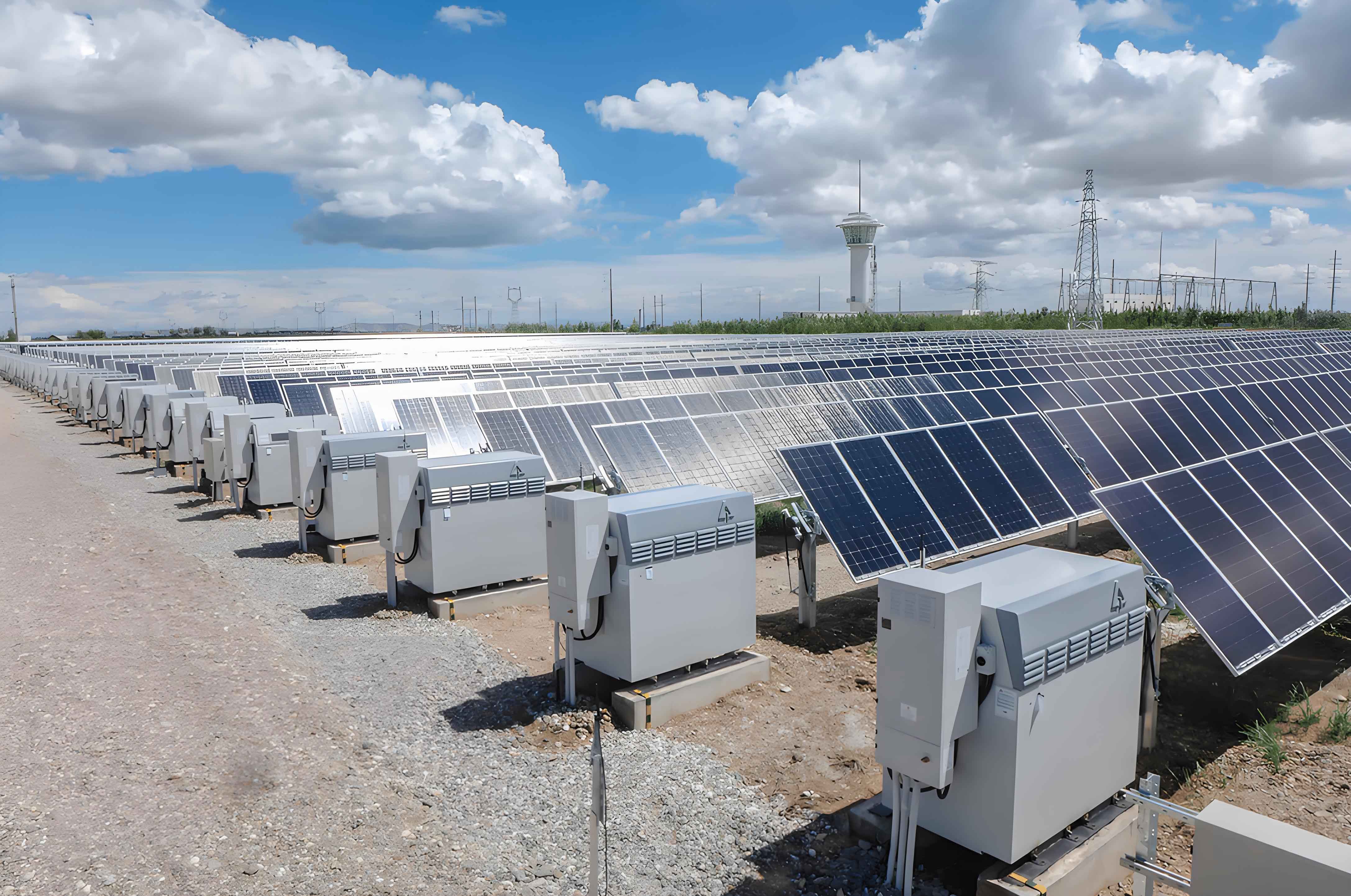
In this study, we propose and validate a novel hierarchical equalization strategy specifically designed for lithium iron phosphate (LFP) energy storage battery systems. Our approach synergistically combines intra-module passive equalization at the cell level with inter-module high-power active equalization. The cornerstone of this architecture is a proprietary Battery Module Equalizer (BME). This device operates not by transferring energy between modules but by intelligently bypassing fully charged or depleted modules during operation, allowing the system to continue charging or discharging the remaining modules until all reach a uniform state of charge (SOC). This method achieves equalization currents commensurate with the main power path (exceeding 300 A), enabling completion within one standard operational cycle. We have conducted extensive Monte Carlo simulations to project long-term benefits and performed rigorous field tests on actual battery clusters to quantify performance gains. The results convincingly demonstrate that our hierarchical equalization system significantly enhances the usable energy of the energy storage battery system, improves consistency, and operates with high efficiency.
Fundamentals of Battery Inconsistency and Equalization
The inconsistency in an energy storage battery pack originates from multiple sources. Initially, there are manufacturing tolerances that lead to slight differences in electrode thickness, electrolyte filling, and active material loading. These result in variances in initial capacity (C) and internal resistance (R). During operation, environmental factors, particularly temperature gradients within the battery enclosure, cause cells to age at different rates. Furthermore, the connection resistances between cells and modules can vary. Over repeated cycles, these small initial differences are amplified, leading to a growing spread in key parameters like capacity, SOC, and impedance. The net effect is a rapid decrease in the system’s usable capacity relative to its theoretical capacity.
The state of a battery cell can be described by its State of Charge (SOC), which is the ratio of its remaining capacity to its maximum available capacity. For a cell i, SOC_i is defined as:
$$SOC_i(t) = SOC_i(0) – \frac{1}{C_i} \int_0^t \eta I(\tau) d\tau$$
where $C_i$ is the capacity of cell i, $I(t)$ is the current (positive for discharge), and $\eta$ is the coulombic efficiency. In a series string of N cells, the pack’s usable capacity is limited by the cell with the minimum capacity or the one that first reaches a voltage boundary. If cells have different capacities $C_1, C_2, …, C_N$, the maximum energy $E_{pack}$ that can be extracted under constant current I is:
$$E_{pack} = V_{nom} \cdot I \cdot \min(C_1, C_2, …, C_N) \cdot \Delta t$$
where $V_{nom}$ is the nominal voltage and $\Delta t$ is the time. Equalization aims to maximize this energy by making the effective $\min(C_i)$ as close as possible to the average capacity.
Traditional equalization methods can be classified by their topology. Passive equalization uses resistive shunts across each cell to bleed off excess charge from higher-SOC cells. The power dissipated $P_{diss}$ for a cell with voltage $V_{cell}$ and shunt current $I_{shunt}$ is:
$$P_{diss} = V_{cell} \cdot I_{shunt}$$
This energy is wasted as heat, and the process is slow because $I_{shunt}$ is small (e.g., 100 mA). For a 280 Ah cell, to reduce a 5% SOC difference (14 Ah), it would take:
$$t_{equalize} = \frac{14 Ah}{0.1 A} = 140 hours$$
which is utterly impractical for daily cycling.
Active equalization methods transfer energy from higher-SOC cells to lower-SOC cells or to/from the whole pack using capacitors, inductors, or transformers. Their efficiency is higher, but the balancing currents are often limited. The energy transfer rate in a typical inductor-based balancer between two adjacent cells is governed by:
$$\Delta E = \frac{1}{2} L (I_{peak}^2)$$
where L is the inductance and $I_{peak}$ is the peak current. Achieving high currents requires large components or high frequencies, increasing cost and complexity. Our analysis of existing systems confirms that currents above 5-10 A are rare, leading to balancing times that still exceed typical cycle durations for large energy storage battery systems.
The Hierarchical Equalization Architecture
Our proposed solution is a two-layer hierarchical system designed for scalability and speed. The first layer operates at the battery module level (typically 18 cells in series). Within each module, a standard passive balancing circuit is employed on the Battery Management Unit (BMU). This handles fine-grained cell-to-cell voltage differences that arise from minor imbalances. The balancing current here is low (e.g., 200 mA), but its continuous operation prevents small variances from accumulating within the module.
The second and most innovative layer is the inter-module active equalization performed by the Battery Module Equalizer (BME). Each battery module in a cluster is equipped with its own BME. The core function of the BME is not to transfer energy but to control the current path through each module via high-power semiconductor switches. The fundamental principle can be illustrated with a simplified circuit model for a module j in a string of M modules.
Let the module voltage be $V_{mj}$ and the string current be $I_{string}$. Each BME contains two main switches, $S_{1j}$ and $S_{2j}$, configured as follows: $S_{1j}$ is in series with the module, and $S_{2j}$ is in parallel with the series combination of $S_{1j}$ and the module. A diode is placed to prevent reverse current. The control logic is SOC-based. The SOC for each module is estimated in real-time by the master BMS using ampere-hour integration combined with voltage correlation for calibration.
During charging, when the BMS determines that module j has reached 100% SOC (while others are still below), it commands the BME for module j to open switch $S_{1j}$ and close switch $S_{2j}$. This action bypasses module j, taking it out of the charging path. The charging current $I_{string}$ now flows through $S_{2j}$, bypassing the module. The remaining modules continue to charge until all reach 100% SOC. The process is analogous during discharge: when a module reaches the minimum allowed SOC (e.g., 10%), it is bypassed, allowing the remaining modules to continue discharging until all reach the cutoff threshold.
The key advantage is the balancing speed. The bypass action is virtually instantaneous, and the “equalization current” is the full system current $I_{string}$, which can be 300 A or more. Therefore, the time to bypass a module is negligible compared to the cycle time. This ensures that all modules are fully utilized in every cycle. The energy loss during bypass is minimal, primarily from the conduction loss of the switch $S_{2j}$, which can be modeled as:
$$P_{loss, bypass} = I_{string}^2 \cdot R_{ds(on)}$$
where $R_{ds(on)}$ is the on-state resistance of the switch, typically a few milliohms for modern MOSFETs or IGBTs.
The overall control strategy for the hierarchical system can be summarized by the following state-based algorithm implemented in the central controller:
Algorithm: Hierarchical SOC-Based Equalization
1. For each module m in cluster, estimate SOC_m(k) at time step k.
2. During CHARGE:
a. Identify set A = {m | SOC_m >= SOC_charge_target}.
b. For all m in A, send command to BME_m: OPEN S1, CLOSE S2 (bypass).
c. For all m not in A, BME_m: CLOSE S1, OPEN S2 (in circuit).
d. Continue until all m have SOC_m >= SOC_charge_target.
3. During DISCHARGE:
a. Identify set B = {m | SOC_m <= SOC_discharge_target}.
b. For all m in B, send command to BME_m: OPEN S1, CLOSE S2 (bypass).
c. For all m not in B, BME_m: CLOSE S1, OPEN S2 (in circuit).
d. Continue until all m have SOC_m <= SOC_discharge_target.
4. Continuously monitor cell voltages within each module; if any cell voltage exceeds a threshold deviation, activate intra-module passive balancing.
This architecture effectively transforms the series string from a “chain limited by the weakest link” into a system where modules can be independently managed, dramatically increasing the usable energy of the energy storage battery cluster.
Monte Carlo Simulation for Long-Term Performance Projection
To quantitatively assess the long-term benefits of our BME-equipped system, we developed a comprehensive Monte Carlo simulation model. The goal was to project the annual energy throughput enhancement over a 10-year operational period, accounting for initial cell capacity distribution, aging effects, and the dynamic equalization process. Monte Carlo methods are ideal for this as they incorporate randomness and uncertainty inherent in battery parameters.
The simulation process is outlined in the flowchart below and involves the following steps mathematically:
1. Initial Capacity Distribution: The capacity of each individual cell is modeled as a random variable following a Gaussian distribution based on production data. For LFP 280 Ah cells, we used a mean $\mu_C = 280 Ah$ and a standard deviation $\sigma_C$ derived from factory grading data (typically 1-2%). Thus, for cell i:
$$C_i^{(0)} \sim \mathcal{N}(\mu_C, \sigma_C^2)$$
2. Module and Cluster Assembly: A battery cluster is composed of 21 modules, each with 18 cells in series (378 cells total). Cells are randomly assigned to modules from the distribution to simulate real-world packing.
3. Aging Model: Capacity fade for each cell is modeled over cycles (years). We used a semi-empirical model where capacity loss increases with cycle number n and is influenced by operational stress factors like temperature and depth of discharge. A simplified version for cell i at year y is:
$$C_i(y) = C_i^{(0)} \cdot (1 – \alpha_i \cdot y^\beta)$$
where $\alpha_i$ is a cell-specific aging rate coefficient (also a random variable, e.g., $\alpha_i \sim \mathcal{N}(\mu_\alpha, \sigma_\alpha^2)$) and $\beta$ is an exponent (often near 0.5 for LFP). The aging rate is also made dependent on the cell’s relative stress; cells that consistently operate at higher SOC extremes may age faster, introducing a positive feedback loop for inconsistency without equalization.
4. Internal Resistance Growth: Similarly, internal resistance $R_i$ increases with aging, affecting voltage divergence under load. We model:
$$R_i(y) = R_i^{(0)} \cdot (1 + \gamma \cdot y)$$
where $\gamma$ is a growth factor.
5. Operational Simulation with and without BME: For each simulated year, we run multiple charge-discharge cycles. For the “without BME” case, the cluster stops charging when the first module’s maximum cell voltage hits the upper limit and stops discharging when the first module’s minimum SOC hits the lower limit. The extractable energy $E_{without}(y)$ is calculated. For the “with BME” case, the BME algorithm is applied, allowing all modules to reach their limits. The energy $E_{with}(y)$ is calculated. The energy gain for year y is:
$$G(y) = E_{with}(y) – E_{without}(y)$$
The percentage gain is:
$$G_{\%}(y) = \frac{G(y)}{E_{without}(y)} \times 100\%$$
6. Monte Carlo Runs: The entire process is repeated for a large number of iterations (e.g., 10,000) to build statistical distributions of the energy gain.
The simulation output provides robust projections. The results are summarized in the following tables for key years.
| Metric | Without BME System | With BME System | Gain |
|---|---|---|---|
| Average Cluster Energy per Cycle (kWh) | 98,150 | 101,244 | 3,094 kWh |
| Standard Deviation (kWh) | 1,250 | 980 | – |
| Minimum Energy (kWh) | 95,200 | 99,800 | – |
| Maximum Energy (kWh) | 101,000 | 102,500 | – |
| Average Energy Gain Percentage | – | – | 3.15% |
| 95% Confidence Interval for Gain % | – | – | [2.95%, 3.35%] |
| Metric | Without BME System | With BME System | Gain |
|---|---|---|---|
| Average Cluster Energy per Cycle (kWh) | 78,450 | 82,507.3 | 4,057.3 kWh |
| Standard Deviation (kWh) | 2,100 | 1,550 | – |
| Minimum Energy (kWh) | 73,500 | 79,200 | – |
| Maximum Energy (kWh) | 82,000 | 84,000 | – |
| Average Energy Gain Percentage | – | – | 5.17% |
| 95% Confidence Interval for Gain % | – | – | [4.88%, 5.46%] |
The cumulative effect over time is even more striking. The simulation allows us to calculate the total additional energy delivered over the lifetime. Let $G_{total}(Y)$ be the cumulative gain over Y years. Assuming 365 equivalent full cycles per year, the cumulative energy gain is:
$$G_{total}(Y) = \sum_{y=1}^{Y} 365 \cdot \bar{G}(y)$$
where $\bar{G}(y)$ is the average annual gain in kWh per cycle from the simulation. The percentage gain relative to the baseline cumulative energy is:
$$G_{total,\%}(Y) = \frac{\sum_{y=1}^{Y} 365 \cdot \bar{G}(y)}{\sum_{y=1}^{Y} 365 \cdot \bar{E}_{without}(y)} \times 100\%$$
Our simulation results for the cumulative performance are summarized below:
| Period | Cumulative Baseline Energy (MWh) | Cumulative Energy with BME (MWh) | Cumulative Gain (MWh) | Cumulative Gain Percentage | Average Annual Gain Percentage |
|---|---|---|---|---|---|
| Years 1-7 | 250.8 | 283.7 | 32.9 | 13.11% | 1.87% |
| Years 1-10 | 286.3 | 373.0 | 86.7 | 30.28% | 3.03% |
The data clearly shows that the hierarchical equalization system not only provides an immediate boost but, crucially, mitigates the accelerating loss of usable capacity over time. The annual gain percentage grows from around 1.5% in early years to over 5% by year 10, underscoring how the system actively counteracts the divergence in cell aging. This has profound implications for the levelized cost of storage (LCOS), as more energy is extracted from the same capital investment in the energy storage battery assets.
Experimental Validation and Field Test Results
Simulations provide theoretical insight, but real-world validation is essential. We deployed our hierarchical equalization system on multiple 2-hour rated energy storage battery clusters at an operational site. Each cluster consisted of 21 battery modules (18 series cells per module, LFP 280 Ah) equipped with our BME units. The clusters were integrated into a containerized energy storage system performing daily charge-discharge cycles for grid peak shaving.
The test protocol involved first operating the clusters for several cycles with the BME function disabled, collecting baseline data on discharge energy, module SOC divergence, and terminal voltages. Subsequently, the BME was enabled, and the same metrics were recorded over an identical number of cycles under similar environmental and load conditions. The primary metric for comparison was the total discharge energy delivered by the cluster from 100% SOC to the system cutoff (approximately 10% SOC minimum).
The improvement in consistency is immediately visible in the voltage and SOC profiles. Without the BME, at the end of charge, the module voltages showed a significant spread, with some modules hitting the upper voltage limit early. With the BME active, all modules were charged fully, resulting in a uniform high voltage profile. A similar effect was observed during discharge. The SOC of all modules at the end of discharge converged to the target (e.g., 10%), whereas without BME, some modules were as high as 15-20% SOC when the discharge terminated due to the weakest module.
Quantitatively, the discharge energy data for 15 tested clusters is presented below. The energy increase is calculated as:
$$\Delta E_{cluster} = E_{discharge, with\ BME} – E_{discharge, without\ BME}$$
$$Increase \% = \frac{\Delta E_{cluster}}{E_{discharge, without\ BME}} \times 100\%$$
Furthermore, we recorded the active working time of the BME during a representative cycle. This is the total time during which one or more modules were in bypass mode. Since the BME only acts when a module hits a limit, its working time is a direct indicator of the level of imbalance and the speed of correction.
| Cluster ID | Discharge Energy without BME (kWh) | Discharge Energy with BME (kWh) | Energy Increase $\Delta E$ (kWh) | Energy Increase Percentage | BME Active Working Time per Cycle (minutes) |
|---|---|---|---|---|---|
| CL-01 | 985.2 | 1010.7 | 25.5 | 2.59% | 10 |
| CL-02 | 972.8 | 1040.5 | 67.7 | 6.96% | 22 |
| CL-03 | 990.1 | 1087.3 | 97.2 | 9.82% | 28 |
| CL-04 | 1001.5 | 1120.8 | 119.3 | 11.91% | 35 |
| CL-05 | 979.3 | 1100.6 | 121.3 | 12.39% | 32 |
| CL-06 | 988.7 | 1095.2 | 106.5 | 10.77% | 30 |
| CL-07 | 995.4 | 1130.9 | 135.5 | 13.61% | 40 |
| CL-08 | 1005.0 | 1155.0 | 150.0 | 14.93% | 45 |
| CL-09 | 987.2 | 1145.1 | 157.9 | 16.00% | 48 |
| CL-10 | 976.5 | 1120.4 | 143.9 | 14.74% | 42 |
| CL-11 | 993.8 | 1115.0 | 121.2 | 12.20% | 31 |
| CL-12 | 1002.3 | 1191.5 | 189.2 | 18.87% | 50 |
| CL-13 | 981.9 | 1102.8 | 120.9 | 12.31% | 33 |
| CL-14 | 989.0 | 1095.5 | 106.5 | 10.77% | 29 |
| CL-15 | 998.1 | 1120.0 | 121.9 | 12.21% | 34 |
| Average | 989.6 | 1107.0 | 117.4 | 10.85% | 26 |
| Std. Dev. | 9.8 | 43.5 | 37.2 | 4.12% | 11.5 |
The results are compelling. The average discharge energy increased by 117.4 kWh per cycle, representing a 10.85% boost. This immediate gain aligns with the simulation’s early-year projections and is directly attributable to recovering the stranded energy in higher-capacity modules. The variation in gain across clusters (2.59% to 18.87%) reflects the differing initial levels of inconsistency; clusters with larger inherent imbalances showed greater improvement.
Critically, the BME active working time averaged only 26 minutes per 2-hour cycle, with a maximum of 50 minutes. This confirms that the equalization process is completed well within a single operational cycle. Compared to a theoretical traditional active balancer with 5 A current trying to correct a 5% SOC imbalance on a 280 Ah module (which requires 2.8 hours as calculated earlier), our system is faster by a factor of:
$$\text{Speed Factor} \approx \frac{2.8\ hours \times 60}{26\ minutes} \approx 6.46$$
In terms of effective balancing current, the BME’s action is equivalent to injecting or removing current at the module level at a rate equal to the system current $I_{string}$. If $I_{string}$ is 300 A, then the effective balancing power is orders of magnitude higher than conventional methods.
The efficiency of the overall process can be estimated. The primary loss mechanisms are the conduction loss in the bypass switch and the energy consumed by the intra-module passive balancers. The bypass loss per module during its bypass time $t_{bypass}$ is:
$$E_{loss, bypass} = I_{string}^2 \cdot R_{ds(on)} \cdot t_{bypass}$$
For a typical $R_{ds(on)} = 2 m\Omega$, $I_{string}=300A$, and $t_{bypass}=26/60 \approx 0.433$ hours (average per cluster, but distributed across modules), the energy loss per cluster per cycle is minimal compared to the energy gain of 117.4 kWh. The system efficiency $\eta_{system}$ considering the gain can be expressed as:
$$\eta_{system} = \frac{E_{delivered, with\ BME}}{E_{delivered, without\ BME} + E_{input, extra}} \approx \text{very high}$$
since the extra energy delivered comes from better utilization of the existing energy storage battery capacity, not from additional input energy.
Mathematical Modeling of the Hierarchical System
To generalize the findings, we can develop a simplified analytical model for the energy gain. Consider a cluster of M modules. Each module j has a capacity $C_j$ (in Ah) and an average voltage $V_{mod}$. Without equalization, the usable capacity is $C_{min} = \min(C_1, C_2, …, C_M)$. With ideal module-level bypass equalization, the usable capacity becomes the sum of the capacities of all modules that can be sequentially used, but in a series string, the voltage adds. However, since bypass effectively allows the system to use the total ampere-hour capacity of the string, the effective usable capacity approaches the average capacity. A more precise model accounts for the fact that during discharge, modules are bypassed one by one as they hit the lower SOC limit.
Let the modules be ordered by their actual capacities such that $C_1 \le C_2 \le … \le C_M$. Without BME, the discharge stops when module 1 is empty. The delivered charge is $Q_{without} = C_1$. With BME, the process is: discharge all modules until module 1 is empty and bypass it; continue discharging modules 2 to M until module 2 is empty and bypass it; and so on. The total delivered charge becomes:
$$Q_{with} = M \cdot C_1 + (M-1) \cdot (C_2 – C_1) + (M-2) \cdot (C_3 – C_2) + … + 1 \cdot (C_M – C_{M-1})$$
This simplifies to:
$$Q_{with} = C_1 + C_2 + … + C_M = \sum_{j=1}^{M} C_j$$
Therefore, the charge gain is:
$$\Delta Q = \sum_{j=1}^{M} C_j – M \cdot C_1 = \sum_{j=2}^{M} (C_j – C_1)$$
The energy gain, assuming average module voltage $V_{mod}$ is constant, is:
$$\Delta E = V_{mod} \cdot \Delta Q = V_{mod} \cdot \sum_{j=2}^{M} (C_j – C_1)$$
If the capacities are normally distributed with mean $\mu_C$ and variance $\sigma_C^2$, then the expected value of $C_1$ (the minimum of M samples) is less than $\mu_C$. The expected gain can be derived using order statistics. For large M, the expected minimum $E[C_1] \approx \mu_C – \Phi^{-1}(\frac{1}{M+1}) \sigma_C$, where $\Phi$ is the normal CDF. Then:
$$E[\Delta Q] \approx M \mu_C – M \cdot E[C_1] \approx M \cdot \Phi^{-1}(\frac{1}{M+1}) \sigma_C$$
This shows that the gain is proportional to the standard deviation of module capacities and the number of modules. This aligns with our simulation and test results: higher initial inconsistency (larger $\sigma_C$) leads to larger gains.
Furthermore, the aging model can be incorporated. If each module’s capacity degrades over time with a random aging factor $\delta_j(y)$, then $C_j(y) = C_j(0) \cdot (1 – \delta_j(y))$. The variance of $C_j(y)$ tends to increase over time because $\delta_j(y)$ are also random, leading to a growing $\Delta Q(y)$, which explains the increasing annual gain percentage in our simulations.
Discussion and Comparative Analysis
The implementation of hierarchical equalization represents a significant leap forward for energy storage battery management. Traditional systems either accept the consistency loss or employ slow equalization that cannot keep pace with operational cycles. Our approach directly attacks the root cause at the module level with a hardware-software co-design that is both effective and efficient.
Compared to pure passive systems, our method eliminates the thermal burden and slowness. While intra-module passive balancing is retained, its role is relegated to managing very fine-grained cell differences, a task for which it is adequate. The major imbalance, which is between modules due to capacity and internal resistance variation, is handled by the high-speed BME.
Compared to conventional active equalization topologies (e.g., switched capacitor, inductor-based, transformer-based), our bypass method offers several advantages:
| Feature | Passive Balancing | Conventional Active Balancing | Proposed Hierarchical BME System |
|---|---|---|---|
| Equalization Current | Low (<1 A) | Medium (1-10 A) | Very High (= System Current, >300 A) |
| Equalization Speed | Very Slow (days) | Slow (hours to days) | Very Fast (minutes, within cycle) |
| Energy Efficiency | Low (energy dissipated as heat) | High (energy transferred) | Very High (minimal conduction loss, no transfer loss) |
| System Complexity | Low | High (many components) | Medium (one BME per module, simple control) |
| Cost | Low | High | Medium (cost of switches & control) |
| Scalability to Large Cells | Poor | Limited | Excellent |
| Ability to Complete Equalization in One Cycle | No | Rarely | Yes |
The economic implication is substantial. For a large-scale energy storage battery plant, a 10% increase in usable energy translates directly to increased revenue from energy arbitrage or ancillary services without increasing the footprint or capital cost of the batteries themselves. Over a 10-year lifetime, the cumulative gain of 30% more energy effectively extends the plant’s economic life or reduces the levelized cost of energy (LCOE) significantly.
From a safety perspective, maintaining tight SOC consistency reduces the risk of individual cells operating outside their safe operating area (SOA). Cells that are consistently undercharged or overcharged relative to others are prone to accelerated degradation and failure modes like lithium plating or thermal runaway. Our system promotes uniform stress across all modules.
Potential limitations and future work include the reliability of the high-power switches over thousands of cycles, the optimization of the control algorithm to further minimize bypass times, and the integration of this approach with other battery health management strategies. We are currently conducting long-term durability tests on the BME hardware. Additionally, the concept can be extended to other battery chemistries beyond LFP, though the voltage profiles and SOC estimation methods would need adaptation.
Conclusion
In conclusion, the inconsistency of lithium-ion batteries remains a fundamental barrier to realizing the full potential of energy storage battery systems. Through this research, we have demonstrated that a hierarchical equalization architecture, combining intra-module passive balancing and inter-module high-power active bypass equalization, provides a highly effective solution. The core innovation, the Battery Module Equalizer, operates with the system’s full current capacity, enabling complete equalization within a single charge-discharge cycle, a feat previously unattainable with existing technologies.
Our Monte Carlo simulations project that this system can deliver an average annual energy boost of approximately 3% over a 10-year period, with cumulative gains exceeding 30%. These projections are strongly corroborated by field tests on actual energy storage battery clusters, which showed an immediate average discharge energy increase of 10.85%, with the equalization process completing in an average of just 26 minutes per 2-hour cycle.
The mathematical models developed confirm that the energy gain is directly related to the variance in module capacities and that the system actively counteracts the positive feedback loop of divergent aging. Compared to traditional methods, our approach offers superior speed, efficiency, and scalability for large-format energy storage battery applications.
This work underscores the importance of innovative battery management strategies in the evolution of grid-scale energy storage. By ensuring that every kilowatt-hour of installed capacity is fully utilizable, hierarchical equalization enhances the economic viability, safety, and longevity of energy storage battery systems, thereby accelerating the integration of renewable energy and the transition to a resilient, low-carbon power grid. Future efforts will focus on long-term operational data collection, cost optimization of the BME hardware, and exploring applications in other storage domains.