
In this work I investigate the complete path from a low-voltage solar panel output to a grid-connected alternating-current supply, and I design a 200 W micro solar inverter around that path. The solar inverter is the central component in a photovoltaic generation system because it converts the direct-current energy produced by photovoltaic modules into alternating-current energy that can be used by local loads or injected into the utility grid. I focus on the interaction among maximum power point tracking, high-frequency voltage step-up, sinusoidal pulse-width modulation, output filtering, and grid-connection control. The design targets a small power rating, low input voltage, stable output waveform, and acceptable total harmonic distortion. Throughout the study I use mathematical models, simulation, and experimental verification to evaluate each stage of the solar inverter.
Background and Motivation
Energy is the foundation of economic development, and the competition among different energy sources has become increasingly intense. Fossil fuels such as oil, natural gas, and coal are finite, and their use creates environmental pollution. Solar energy is abundant, clean, and widely distributed. It can be converted into electricity locally and can be combined with different residential and industrial usage patterns. Among renewable sources, solar energy has a unique advantage because it is effectively inexhaustible and does not require fuel transportation or combustion. For these reasons, photovoltaic generation has become one of the most important directions in new energy development.
A typical photovoltaic generation system includes a solar panel array, a controller, a solar inverter, and possibly a battery or grid interface. The solar panel converts light into electricity. The controller performs maximum power point tracking, protection, and modulation. The solar inverter performs direct-current to alternating-current conversion. In grid-connected operation, the solar inverter must synchronize its output current with the grid voltage and maintain power quality. The efficiency, stability, and harmonic performance of the solar inverter directly affect the overall energy yield of the photovoltaic system.
I reviewed the development of photovoltaic systems and solar inverter products. Early photovoltaic systems were mainly used in remote areas where grid extension was expensive. With advances in power semiconductors and digital signal processors, grid-connected solar inverter systems have become more compact and more efficient. High-frequency switching, transformer isolation, and advanced control algorithms have made micro solar inverter designs practical for module-level power conversion. The research presented here is motivated by the need for a small, efficient, and reliable solar inverter that can operate from a 24 V direct-current source and produce a 220 V, 50 Hz alternating-current output.
| Item | Description | Relevance to the Solar Inverter |
|---|---|---|
| Energy source | Solar radiation | Determines the input power available to the solar inverter |
| Conversion device | Photovoltaic module | Produces low-voltage direct current |
| Core power stage | DC-DC step-up and DC-AC inversion | Main power conversion inside the solar inverter |
| Control platform | Digital signal processor | Generates PWM and SPWM signals for the solar inverter |
| Grid interface | Current-controlled connection | Ensures the solar inverter feeds the grid with acceptable current quality |
Maximum Power Point Tracking for the Solar Inverter
Maximum power point tracking is essential for a solar inverter because the output power of a photovoltaic module varies with irradiance, temperature, load, and aging. If the solar inverter does not track the maximum power point, the available solar energy is not fully utilized. I therefore began by analyzing the electrical behavior of the solar cell and then developed a tracking method that improves both speed and accuracy.
Solar Cell Operating Principle and Model
A solar cell is essentially a large-area p-n junction. When photons with sufficient energy strike the semiconductor, electron-hole pairs are generated. The internal electric field of the depletion region separates these carriers, producing a photocurrent. When an external load is connected, the cell delivers electrical power. The equivalent circuit includes a current source, a diode, a series resistance, and a shunt resistance. The current-voltage relationship can be written as
$$I = I_L – I_D \left( e^{\frac{q(V + I R_s)}{n k T}} – 1 \right) – \frac{V + I R_s}{R_{sh}}$$
where \(I_L\) is the photocurrent, \(I_D\) is the diode saturation current, \(q\) is the electron charge, \(V\) is the terminal voltage, \(n\) is the diode ideality factor, \(k\) is the Boltzmann constant, \(T\) is the absolute temperature, \(R_s\) is the series resistance, and \(R_{sh}\) is the shunt resistance. This equation is the basis for the photovoltaic model used in my simulation of the solar inverter input stage.
For a practical photovoltaic module, the parameters are usually given at a reference temperature and irradiance. I used a simulation model in which the short-circuit current, open-circuit voltage, maximum power point voltage, and maximum power point current can be adjusted. The model allows the irradiance and temperature to be varied so that the effect on the solar inverter input can be observed.
| Parameter | Meaning | Effect on the Solar Inverter |
|---|---|---|
| Open-circuit voltage | Voltage at zero current | Sets the upper input voltage limit |
| Short-circuit current | Current at zero voltage | Sets the maximum input current |
| Maximum power point voltage | Voltage at maximum power | Target operating point for the solar inverter |
| Maximum power point current | Current at maximum power | Determines the current stress in the input stage |
| Temperature coefficient | Change per degree Celsius | Shifts the maximum power point as the module heats |
| Irradiance | Incident solar power per unit area | Scales the available current and power |
Simulation results showed that the current-voltage curve and the power-voltage curve change with temperature and irradiance. At a fixed irradiance, increasing temperature reduces the open-circuit voltage and slightly increases the short-circuit current, but the net effect is a reduction in maximum power. At a fixed temperature, increasing irradiance increases both current and power. The power-voltage curve is approximately parabolic near its peak, and there is a unique maximum power point for a given set of conditions. This means that the solar inverter must continuously adjust its operating point.
Conventional MPPT Methods
Several maximum power point tracking methods are commonly used in solar inverter systems. The constant-voltage method assumes that the maximum power point voltage is a fixed fraction of the open-circuit voltage. It is simple and inexpensive, but it does not respond well to temperature changes. The perturbation-and-observation method periodically perturbs the operating voltage and observes the resulting power change. If power increases, the perturbation continues in the same direction; if power decreases, the direction is reversed. This method is easy to implement, but a fixed perturbation step creates a trade-off between tracking speed and steady-state oscillation. A large step gives fast tracking but causes power oscillation around the maximum power point. A small step reduces oscillation but slows the response.
| Method | Principle | Advantages | Limitations |
|---|---|---|---|
| Constant-voltage | Hold a fixed fraction of open-circuit voltage | Simple, low cost | Poor temperature response, low accuracy |
| Perturbation and observation | Perturb voltage and observe power | Simple, widely used | Oscillation and speed trade-off |
| Incremental conductance | Use \(dP/dV = 0\) condition | Good accuracy, less oscillation | Fixed step still limits speed |
| Variable-step incremental conductance | Adapt step to slope of power curve | Fast and accurate | More computation |
Variable-Step Incremental Conductance Algorithm
The incremental conductance method uses the fact that the derivative of power with respect to voltage is zero at the maximum power point. Starting from
$$P = V I$$
the derivative is
$$\frac{dP}{dV} = I + V \frac{dI}{dV}$$
At the maximum power point,
$$\frac{dP}{dV} = 0$$
so
$$\frac{I}{V} + \frac{dI}{dV} = 0$$
Here \(I/V\) is the instantaneous conductance and \(dI/dV\) is the incremental conductance. By comparing the sum of these two terms with zero, the solar inverter controller can decide whether to increase or decrease the operating voltage. A conventional incremental conductance algorithm still uses a fixed voltage step, which creates the same speed-accuracy conflict as the perturbation-and-observation method.
I proposed a variable-step incremental conductance algorithm for the solar inverter. The step size is adjusted according to the slope of the power-voltage curve. When the operating point is far from the maximum power point, the slope is large and the step size is increased. When the operating point is close to the maximum power point, the slope is small and the step size is reduced. This improves tracking speed while avoiding steady-state oscillation. In addition, I included a fixed maximum step limit to prevent the operating voltage from jumping outside the safe range when irradiance or temperature changes abruptly.
The algorithm can be summarized as follows. The controller samples the present voltage \(V_n\) and current \(I_n\). It calculates the differences
$$\Delta V = V_n – V_{n-1}$$
$$\Delta I = I_n – I_{n-1}$$
If \(\Delta V \neq 0\), the controller evaluates the incremental conductance condition. If the sum \(I/V + dI/dV\) is positive, the voltage reference is increased. If the sum is negative, the voltage reference is decreased. If the sum is zero, the operating point is at the maximum power point and the reference is held. The voltage step is
$$\Delta V_{ref} = K \left| \frac{I}{V} + \frac{dI}{dV} \right|$$
where \(K\) is a scaling factor. To prevent excessive steps, the step is limited by
$$\Delta V_{ref} \leq \Delta V_{\max}$$
This variable-step approach was tested in simulation. The conventional incremental conductance method showed a longer settling time and small oscillations around the maximum power point. The variable-step method reached the maximum power point faster and then remained stable. The improvement is important for a solar inverter because it directly increases the average power extracted from the photovoltaic module.
Solar Inverter Topology and Overall Design
The micro solar inverter studied here has a two-stage structure because the input voltage from a single photovoltaic module is much lower than the peak voltage required for a 220 V alternating-current output. The first stage steps up the low direct-current voltage through a high-frequency transformer. The second stage inverts the high direct-current voltage into a sinusoidal alternating-current output and filters it before connection to the grid. The overall system block includes the photovoltaic source, the step-up stage, the inverter bridge, the output filter, the digital controller, and the measurement circuits.
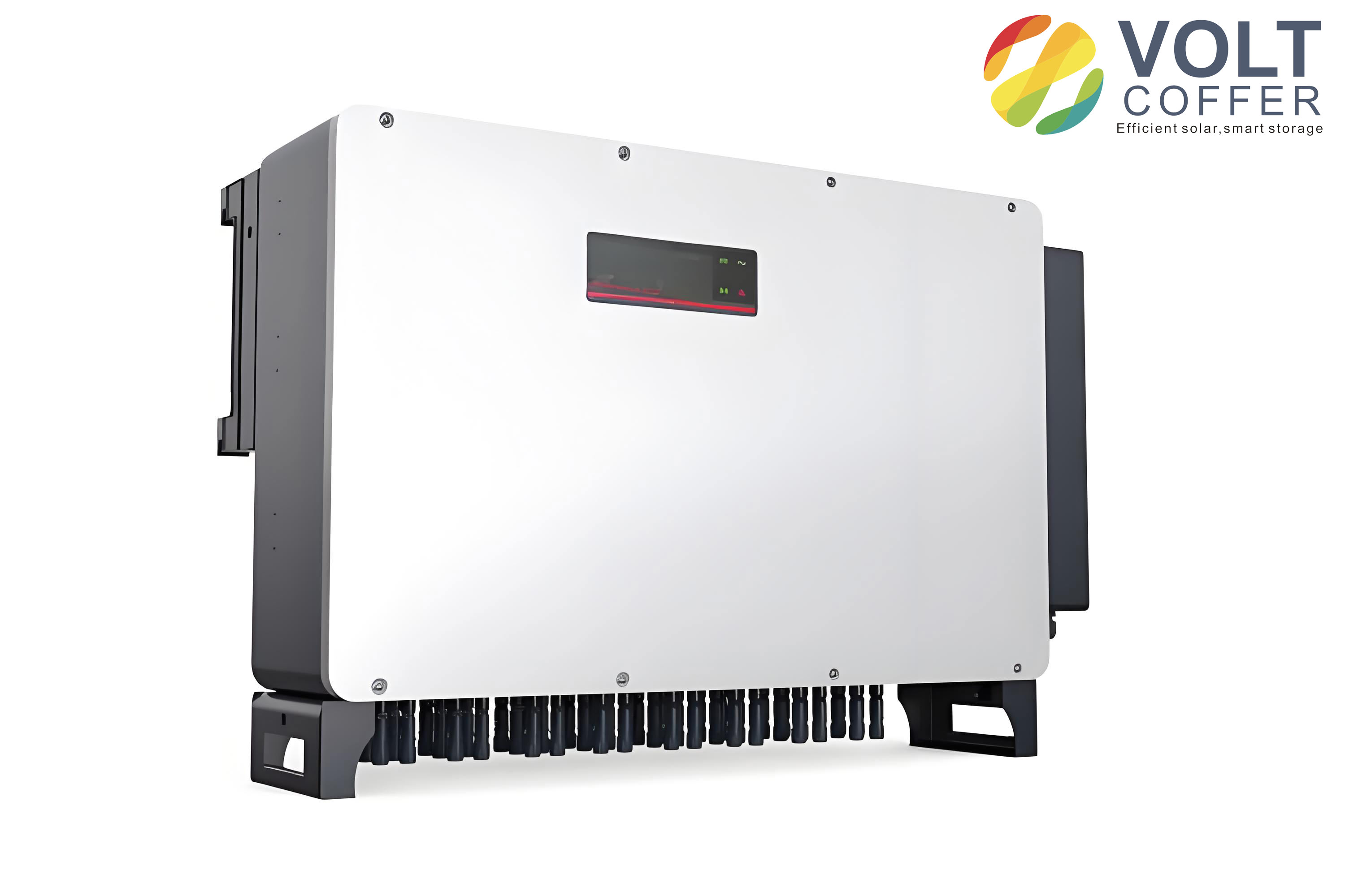
The controller is responsible for maximum power point tracking, pulse-width modulation for the step-up stage, sinusoidal pulse-width modulation for the inverter bridge, over-voltage protection, under-voltage protection, over-current protection, and grid synchronization. I selected a digital signal processor as the control platform because it can execute floating-point operations quickly and can generate multiple high-resolution PWM channels. The solar inverter power stage was designed for a nominal input of 24 V and an output of 200 W.
| Specification | Target Value | Notes |
|---|---|---|
| Input rated voltage | 24 V DC | Low-voltage photovoltaic module |
| Output voltage RMS | 220 V ± 5% | Alternating-current grid interface |
| Output frequency | 50 Hz ± 5% | Grid-compatible frequency |
| Output power | 200 W | Micro solar inverter rating |
| Total harmonic distortion | Below 5% | Grid current quality requirement |
| Conversion efficiency | About 85% | Target for the complete solar inverter |
Push-Pull Step-Up Stage
For the first stage I used a push-pull converter. Two power switches are driven alternately by a high-frequency PWM signal. The transformer primary is center-tapped, and the secondary winding feeds a rectifier and a direct-current link capacitor. The push-pull topology is suitable for low-voltage input because only one switch is in the conduction path at a time, reducing conduction loss. The transformer also provides galvanic isolation, which is desirable for a solar inverter that may be connected to a grounded grid.
The switching frequency was chosen as 50 kHz. The duty cycle was set to about 45% with a small dead time to prevent simultaneous conduction of the two switches. The input current is large because the input voltage is low. For a 200 W solar inverter operating from 24 V, the average input current is approximately 8.3 A, and the peak current can be higher. I selected MOSFETs with low on-resistance and adequate voltage and current margins. The gate driver provides the required drive voltage and isolation.
$$I_{in,avg} = \frac{P_{out}}{\eta V_{in}}$$
For \(P_{out} = 200\) W, \(\eta = 0.85\), and \(V_{in} = 24\) V, the average input current is approximately 9.8 A. This confirms that the input stage must be designed for high current and low conduction loss.
Full-Bridge Inverter Stage
The second stage is a full-bridge inverter. Four power switches form two bridge legs. The load or grid is connected between the midpoints of the two legs through an output filter. Compared with a half-bridge inverter, the full-bridge inverter applies the full direct-current link voltage across the output, so the output current for the same power is lower. This reduces current stress and conduction loss. The full-bridge topology is therefore a good match for the 200 W solar inverter design.
The switches are controlled by sinusoidal pulse-width modulation. The modulation signal is a 50 Hz sine wave, and the carrier is a 30 kHz triangular wave. The resulting SPWM signal drives the bridge so that the output voltage contains a fundamental component at 50 Hz and high-frequency harmonic components. The output filter removes most of the high-frequency content and leaves a nearly sinusoidal voltage for the grid interface.
SPWM Generation and Control
Sinusoidal pulse-width modulation is based on the principle of equal impulse. A sine wave is divided into many narrow pulses. Each pulse has equal amplitude but different width, and the width follows the sine law. When the pulse train is applied to the inverter bridge, the fundamental component resembles the original sine wave, while the high-frequency components are filtered. The modulation index and the frequency ratio determine the harmonic spectrum of the solar inverter output.
The modulation index is
$$M = \frac{U_{sm}}{U_r}$$
and the frequency ratio is
$$N = \frac{f_r}{f_s}$$
where \(U_{sm}\) is the sine wave amplitude, \(U_r\) is the carrier amplitude, \(f_r\) is the carrier frequency, and \(f_s\) is the modulation frequency. The output fundamental voltage of the full-bridge solar inverter is approximately
$$U_{ab,1} = \frac{M U_d}{2} \sin(\omega_s t + \phi)$$
where \(U_d\) is the direct-current link voltage. The harmonic frequencies are located around multiples of the carrier frequency, and their amplitudes depend on Bessel functions of the modulation index.
Sampling Methods for SPWM
Digital generation of SPWM requires a sampling method. The natural sampling method uses the exact intersections of the sine wave and the triangular carrier. Although it gives the best harmonic performance, it requires solving a transcendental equation, which is difficult in a real-time controller. The symmetrical regular sampling method samples the sine wave at the carrier peak or valley. The switching instants are symmetric about the carrier valley or peak, and the pulse width can be calculated with a simple equation. The asymmetrical regular sampling method samples at both the carrier peak and valley, giving better accuracy but requiring more computation.
| Sampling Method | Sampling Instant | Computation | Harmonic Performance |
|---|---|---|---|
| Natural sampling | Exact intersections | Very high | Best |
| Symmetrical regular sampling | Carrier peak or valley | Low | Good |
| Asymmetrical regular sampling | Carrier peak and valley | Medium | Better than symmetrical |
For the symmetrical regular sampling method, the on-time is
$$t_{on} = \frac{T_s}{4} \left( 1 + M \sin(\omega_s t_1) \right)$$
where \(T_s\) is the carrier period and \(t_1\) is the sampling instant. For the asymmetrical regular sampling method, the on-time is
$$t_{on} = \frac{T_s}{4} \left[ 1 + \frac{M}{2} \left( \sin(\omega_s t_1) + \sin(\omega_s t_2) \right) \right]$$
where \(t_1\) and \(t_2\) are the sampling instants at the carrier peak and valley. The natural sampling method requires solving
$$t = \frac{T_s}{4} \left[ 1 + \frac{M}{2} \left( \sin(\omega_s t_1) + \sin(\omega_s t_2) \right) \right]$$
which is an implicit equation. Because the symmetrical regular sampling method is simple and accurate enough for the solar inverter, I used it in the digital implementation.
Bipolar, Unipolar, and Double-Frequency SPWM
SPWM can be classified as bipolar, unipolar, or double-frequency. In bipolar modulation, the output voltage of the inverter leg switches between positive and negative direct-current link voltage. In unipolar modulation, the output voltage switches between zero and either positive or negative voltage. Double-frequency SPWM uses one bridge leg controlled by a sine wave compared with a triangular carrier, and the other leg controlled by the same sine wave compared with an inverted triangular carrier or by an inverted sine wave compared with the same carrier. The result is that the effective switching frequency of the output voltage is doubled. This pushes the dominant harmonics to higher frequencies, where they are easier to filter.
I analyzed the harmonic content of the full-bridge solar inverter under double-frequency SPWM. The output voltage can be expressed as a Fourier series. For a half-bridge circuit, the output voltage with bipolar SPWM has the form
$$U_{ao} = \frac{U_d}{2} + \sum_{n=1}^{\infty} a_n \cos(n \omega_c t)$$
where the coefficients depend on the switching angles. For the full-bridge inverter with double-frequency SPWM, the harmonic frequencies are
$$n \omega_c \pm k \omega_s$$
and the harmonic amplitudes are
$$A_{n,k} = \frac{4 U_d}{n \pi} J_k \left( \frac{n \pi M}{2} \right)$$
for even \(n\) and odd \(k\). This shows that the low-order harmonics are greatly reduced and the remaining harmonics are concentrated around the carrier frequency and its multiples. The output filter can therefore be designed to attenuate these high-frequency components effectively.
Output Filter Design for the Solar Inverter
The unfiltered output of the full-bridge solar inverter is a train of high-frequency pulses whose width varies sinusoidally. A low-pass filter is needed to extract the 50 Hz fundamental and suppress the switching harmonics. A simple LC filter is often used, but I found that load variations can cause the output waveform to become less stable and the total harmonic distortion to increase. I therefore investigated an LC-LC series filter for the solar inverter output.
For a simple LC filter, the inductor value is chosen according to the maximum ripple current. The ripple current is
$$\Delta I_L = \frac{U_d – U_o}{L} \frac{U_o}{U_d f_c}$$
The maximum ripple occurs when \(U_o = U_d/2\). The inductor must satisfy
$$L \geq \frac{U_d}{4 f_c \Delta I_L}$$
The cutoff frequency of the LC filter is
$$f_c = \frac{1}{2 \pi \sqrt{L C}}$$
In practice, the cutoff frequency is placed well below the lowest significant harmonic frequency and well above the fundamental frequency. For a 200 W solar inverter with a 400 V direct-current link, a modulation frequency of 50 Hz, and a carrier frequency of 30 kHz, the lowest significant harmonic is around 30 kHz. I chose a cutoff frequency of about 3 kHz.
| Filter Parameter | Value | Design Basis |
|---|---|---|
| First inductor \(L_1\) | 1.68 mH | Ripple current limit |
| Second inductor \(L_2\) | 16.8 mH | High-frequency attenuation |
| First capacitor \(C_1\) | 1.4 μF | Cutoff frequency |
| Second capacitor \(C_2\) | 1.68 μF | Output smoothing |
| Cutoff frequency | 3 kHz | Between fundamental and carrier |
The LC-LC filter transfer function can be written as
$$\frac{U_o(s)}{U_i(s)} = \frac{1}{a s^4 + b s^3 + c s^2 + d s + 1}$$
where the coefficients depend on the inductances, capacitances, and load resistance. When the load resistance is large enough, the transfer function can be simplified. In the design I set \(L_1 = L_2/10\) and tuned the capacitors to obtain a smooth response for both heavy and light loads. Simulation with a 200 Ω load and a 10 Ω load showed that the output waveform remained stable and that the total harmonic distortion was about 0.96%, which is well below the 5% requirement.
Grid-Connection Control Strategies for the Solar Inverter
A grid-connected solar inverter must deliver current that is synchronized with the grid voltage. The grid behaves as a large voltage source with fluctuating amplitude and frequency. If the solar inverter is controlled as a voltage source, grid voltage disturbances can strongly affect the output current and degrade power quality. Therefore, current control is usually preferred. In current control, the solar inverter behaves as a current source, and the output current is regulated to follow a reference sine wave that is synchronized with the grid voltage.
I studied three current-control strategies: hysteresis current control, proportional-integral control, and deadbeat control. Each has advantages and limitations for a solar inverter.
Hysteresis Current Control
Hysteresis current control compares the actual grid current with a reference current. The error is fed to a hysteresis comparator with a specified band. When the error exceeds the upper limit, the inverter switches to increase the current. When the error falls below the lower limit, the inverter switches to decrease the current. The switching frequency is not fixed; it depends on the inductance, the direct-current link voltage, and the hysteresis band.
The main advantage of hysteresis current control is its simplicity and fast response. It does not require an accurate system model. However, the variable switching frequency makes filter design difficult and increases switching losses. A narrow hysteresis band improves current accuracy but raises the switching frequency. A wide band reduces switching losses but increases harmonic distortion.
| Feature | Hysteresis Current Control | PI Control | Deadbeat Control |
|---|---|---|---|
| Model dependence | Low | Medium | High |
| Switching frequency | Variable | Fixed | Fixed |
| Response speed | Fast | Moderate | Very fast |
| Harmonic performance | Depends on band | Good | Excellent |
| Implementation complexity | Low | Medium | High |
PI Control
Proportional-integral control is widely used in industrial systems. For the solar inverter, the grid current is sampled and compared with a reference current. The error is processed by a PI regulator, and the output is used as the modulation signal for SPWM generation. The transfer function of the PI regulator is
$$G_3(s) = k_p + \frac{k_i}{s}$$
The inverter bridge can be approximated as a gain \(G_2(s) = k_{spwm}\). The output filter and grid inductance introduce a transfer function \(G_1(s)\). The closed-loop current response depends on these transfer functions. If the grid voltage is considered as a disturbance, the influence of the grid voltage on the grid current can be reduced by adding a feedforward compensation term. The condition for eliminating the grid voltage effect is
$$G_4(s) = \frac{1}{G_2(s)}$$
With proper feedforward, the solar inverter current becomes less sensitive to grid voltage fluctuations. Simulation showed that PI control with feedforward produced a clean sinusoidal current and good harmonic performance. The main disadvantage is that the control parameters must be tuned for the expected grid inductance and operating point.
Deadbeat Control
Deadbeat control is a digital control method that calculates the required switching duty cycle for the next sampling period based on the measured current and the system model. For the grid-connected solar inverter, the circuit equation is
$$L \frac{d i_L}{dt} = U_{ab} – U_{ac} – R i_L$$
Discretizing this equation over one sampling period gives
$$U_{ab}(k) = \frac{L}{T_s} \left( i_L(k+1) – i_L(k) \right) + R i_L(k) + U_{ac}(k)$$
The duty cycle for the inverter bridge is then
$$D(k) = \frac{1}{U_{dc}} \left[ \frac{L}{T_s} \left( i_{ref}(k+1) – i_L(k) \right) + R i_L(k) + U_{ac}(k) \right]$$
Deadbeat control has a very fast dynamic response and can achieve excellent current tracking if the model is accurate. However, it is sensitive to parameter errors and measurement noise. In a low-cost solar inverter, the additional computation and model dependence may not be justified.
After comparing the three strategies, I selected PI control with feedforward for the grid-connected solar inverter. It provides a good balance between implementation complexity, harmonic performance, and robustness against grid voltage variations.
System Implementation
The complete solar inverter prototype includes the input filter, push-pull step-up stage, high-frequency transformer, rectifier, direct-current link capacitor, full-bridge inverter, output filter, gate drivers, measurement circuits, and digital controller. The power stage was built on a printed circuit board with careful attention to grounding and thermal management. The control board is based on a digital signal processor with multiple enhanced PWM modules.
Hardware Design Details
The input capacitor reduces the voltage ripple from the photovoltaic source. The push-pull switches are driven by a high-frequency PWM signal generated by the digital signal processor. The transformer turns ratio is chosen so that the rectified direct-current link voltage is high enough to produce a 220 V alternating-current output with some margin. The full-bridge switches are driven by SPWM signals with a 30 kHz carrier and a 50 Hz modulation wave. The output filter uses the LC-LC configuration described earlier.
| Stage | Component | Key Rating | Function in the Solar Inverter |
|---|---|---|---|
| Input | Electrolytic capacitor | Low ESR, 50 V | Smoothes the photovoltaic input |
| Step-up | MOSFET | 200 V, 18 A | Push-pull switching |
| Step-up | High-frequency transformer | 50 kHz, ferrite core | Voltage step-up and isolation |
| Rectifier | Fast recovery diodes | 600 V, 3 A | Rectifies the transformer secondary |
| Inverter | IGBT or MOSFET | 1200 V, 20 A | Full-bridge SPWM inversion |
| Filter | Inductors and capacitors | As designed | Attenuates switching harmonics |
| Control | Digital signal processor | 150 MHz, floating point | MPPT, PWM, SPWM, protection |
Software Design
The software for the solar inverter is organized around the enhanced PWM modules of the digital signal processor. Each module includes a time-base unit, a counter-compare unit, an action-qualifier unit, a dead-band unit, a chopper unit, an event-trigger unit, and a trip-zone unit. The time-base unit sets the switching frequency. The counter-compare unit sets the duty cycle. The action-qualifier unit determines the output polarity. The dead-band unit inserts the required dead time to prevent shoot-through in the full-bridge inverter.
The main program performs system initialization, configures the PWM and SPWM modules, calculates the sine table, enables interrupts, and then enters a loop. In the interrupt service routine, the controller updates the compare registers with new duty-cycle values, clears the interrupt flag, and returns. The maximum power point tracking algorithm runs at a slower rate than the SPWM update because the photovoltaic operating point changes relatively slowly. The protection routines monitor input voltage, input current, output voltage, output current, and temperature.
| Software Task | Execution Rate | Purpose |
|---|---|---|
| SPWM update | 30 kHz | Generate inverter bridge gate signals |
| PWM update for step-up | 50 kHz | Drive push-pull switches |
| MPPT calculation | 100 Hz | Track the maximum power point |
| Protection scan | 10 kHz | Detect fault conditions |
| Grid synchronization | 10 kHz | Lock the output current to the grid voltage |
Experimental Results
The prototype solar inverter was tested with a 24 V direct-current source and a resistive load. The SPWM signal from the digital signal processor was observed, and the output voltage after the full-bridge inverter and LC-LC filter was measured. The output waveform was stable and nearly sinusoidal. The fundamental frequency was 50 Hz, and the total harmonic distortion was low. The output power was approximately 200 W, and the conversion efficiency was about 85%.
| Measured Quantity | Result | Requirement |
|---|---|---|
| Input voltage | 24 V DC | 24 V nominal |
| Output voltage RMS | 220 V | 220 V ± 5% |
| Output frequency | 50 Hz | 50 Hz ± 5% |
| Output power | 200 W | 200 W |
| Total harmonic distortion | About 0.96% | Below 5% |
| Conversion efficiency | About 85% | Target about 85% |
The experimental results confirm that the push-pull step-up stage, the full-bridge inverter, the double-frequency SPWM, and the LC-LC output filter work together to produce a high-quality alternating-current output. The variable-step incremental conductance algorithm keeps the solar inverter operating near the maximum power point even when the input conditions change. The digital controller provides the required flexibility for protection and future grid-connection features.
Discussion of Key Design Trade-Offs
The design of a solar inverter involves several trade-offs. Increasing the switching frequency reduces the size of the transformer and filter but increases switching losses and electromagnetic interference. Increasing the direct-current link voltage reduces current stress but requires higher-voltage semiconductors and more careful insulation. Increasing the filter order improves harmonic attenuation but adds cost, weight, and possible resonance. The variable-step MPPT improves energy capture but requires more computation. The grid-connection control strategy affects current quality, stability, and robustness. In my design I balanced these factors to achieve a compact 200 W solar inverter with acceptable efficiency and power quality.
| Design Choice | Benefit | Cost or Risk |
|---|---|---|
| High switching frequency | Smaller magnetics and filter | Higher switching loss |
| Push-pull step-up | Low input current stress | Transformer saturation risk |
| Full-bridge inverter | Lower output current stress | More switches and drivers |
| Double-frequency SPWM | Higher effective harmonic frequency | More complex modulation logic |
| LC-LC filter | Stable output under load change | More components and possible resonance |
| Variable-step MPPT | Faster and more accurate tracking | Higher computation load |
| PI grid control | Good balance of simplicity and performance | Requires parameter tuning |
Further Analysis of Harmonic Performance
The harmonic performance of the solar inverter is determined by the modulation method and the output filter. Double-frequency SPWM shifts the dominant harmonics to twice the carrier frequency and its sidebands. The first significant harmonic group appears near \(2 f_c\), where \(f_c\) is the carrier frequency. For a 30 kHz carrier, the first group is near 60 kHz. The LC-LC filter attenuates this group strongly because its cutoff frequency is much lower. The remaining low-order harmonics are mainly caused by dead time, device voltage drops, and grid voltage distortion. Careful dead-time compensation and accurate current control reduce these effects.
The total harmonic distortion of the output current can be estimated from the harmonic amplitudes and the filter attenuation. If the harmonic voltage at frequency \(f_h\) is \(U_h\), the harmonic current is approximately
$$I_h = \frac{U_h}{Z(f_h)}$$
where \(Z(f_h)\) is the filter and grid impedance at the harmonic frequency. The total harmonic distortion is
$$THD = \sqrt{\sum_{h=2}^{\infty} \left( \frac{I_h}{I_1} \right)^2}$$
where \(I_1\) is the fundamental current. My simulation and measurement showed that the LC-LC filter reduces the total harmonic distortion to about 0.96%, which is well within the grid-connection requirement.
Maximum Power Point Tracking Performance
The variable-step incremental conductance algorithm was evaluated under step changes in irradiance and temperature. The algorithm adjusts the operating voltage quickly when the power curve slope is large. Near the maximum power point, the step size becomes small, so the operating point does not oscillate. The fixed-step method showed a persistent small oscillation around the maximum power point, which wastes a small amount of available energy. The variable-step method reduced this oscillation and improved the average output power. For a solar inverter, even a small improvement in MPPT efficiency can increase the total energy yield over a day.
| Condition | Fixed-Step MPPT | Variable-Step MPPT |
|---|---|---|
| Start-up tracking time | Longer | Shorter |
| Steady-state oscillation | Noticeable | Very small |
| Response to irradiance change | Moderate | Fast |
| Computation load | Low | Moderate |
| Average power capture | Good | Better |
Grid-Connection Considerations
For a grid-connected solar inverter, the output current must be synchronized with the grid voltage. The controller uses a phase-locked loop or a zero-crossing detector to obtain the grid phase. The reference current is generated as a sine wave in phase with the grid voltage. The amplitude of the reference current is set by the available photovoltaic power and the direct-current link voltage. The current control loop then adjusts the inverter duty cycle to make the actual current follow the reference. Protection functions include anti-islanding detection, over-voltage, under-voltage, over-frequency, under-frequency, and over-current protection.
In my study I focused on the current-control inner loop. The PI controller with feedforward gave good results. The hysteresis controller was simple but produced variable switching frequency. The deadbeat controller was fast but sensitive to model errors. For a practical solar inverter, a combination of PI control and feedforward is a reasonable choice. Future work can add anti-islanding and grid-support functions.
Conclusion and Future Work
I have presented the research and design of a 200 W grid-connected micro solar inverter. The solar inverter uses a two-stage topology: a push-pull step-up stage with a high-frequency transformer and a full-bridge inverter stage with double-frequency SPWM. The input is a 24 V direct-current source, and the output is a 220 V, 50 Hz alternating-current supply. The variable-step incremental conductance algorithm improves maximum power point tracking by adapting the voltage step to the slope of the power-voltage curve. The LC-LC output filter reduces the total harmonic distortion to about 0.96% and maintains a stable output waveform under load changes. The digital signal processor generates the PWM and SPWM signals, performs MPPT, and implements protection. Experimental results show that the solar inverter delivers about 200 W with an efficiency of about 85% and meets the harmonic requirement.
Future work should focus on several areas. First, a more advanced MPPT algorithm can be developed to handle partial shading and rapidly changing irradiance. Second, the solar inverter efficiency can be improved by using soft-switching techniques and better magnetic components. Third, the grid-connection control can be extended with anti-islanding detection, reactive power support, and communication functions. Fourth, the thermal design and electromagnetic compatibility can be optimized for a more compact product. Finally, the solar inverter can be integrated with energy storage and smart-grid interfaces to increase its value in distributed generation systems.
The work confirms that careful modeling, simulation, and experimental verification are essential for a successful solar inverter design. The interaction among the photovoltaic source, the power stage, the filter, and the control algorithm determines the final performance. By improving each of these elements, a small solar inverter can achieve high power quality and reliable operation.