
In my research, I focus on GaN-based micro solar inverters because they sit at the intersection of two important trends: the rapid growth of distributed photovoltaic generation and the demand for power converters with higher frequency, higher power density, and smaller volume. Solar inverters are no longer only large central devices placed in utility-scale plants. They are increasingly distributed at the module level, where each photovoltaic panel can have its own conversion channel. In my view, micro solar inverters are especially attractive for building-integrated photovoltaics, rooftop systems, and locations with partial shading, because module-level conversion can reduce mismatch losses and improve the total energy harvest. The use of GaN high-electron-mobility transistors in these solar inverters allows switching frequencies far beyond those commonly used in silicon-based designs, which directly reduces passive component size and makes compact integration more feasible.
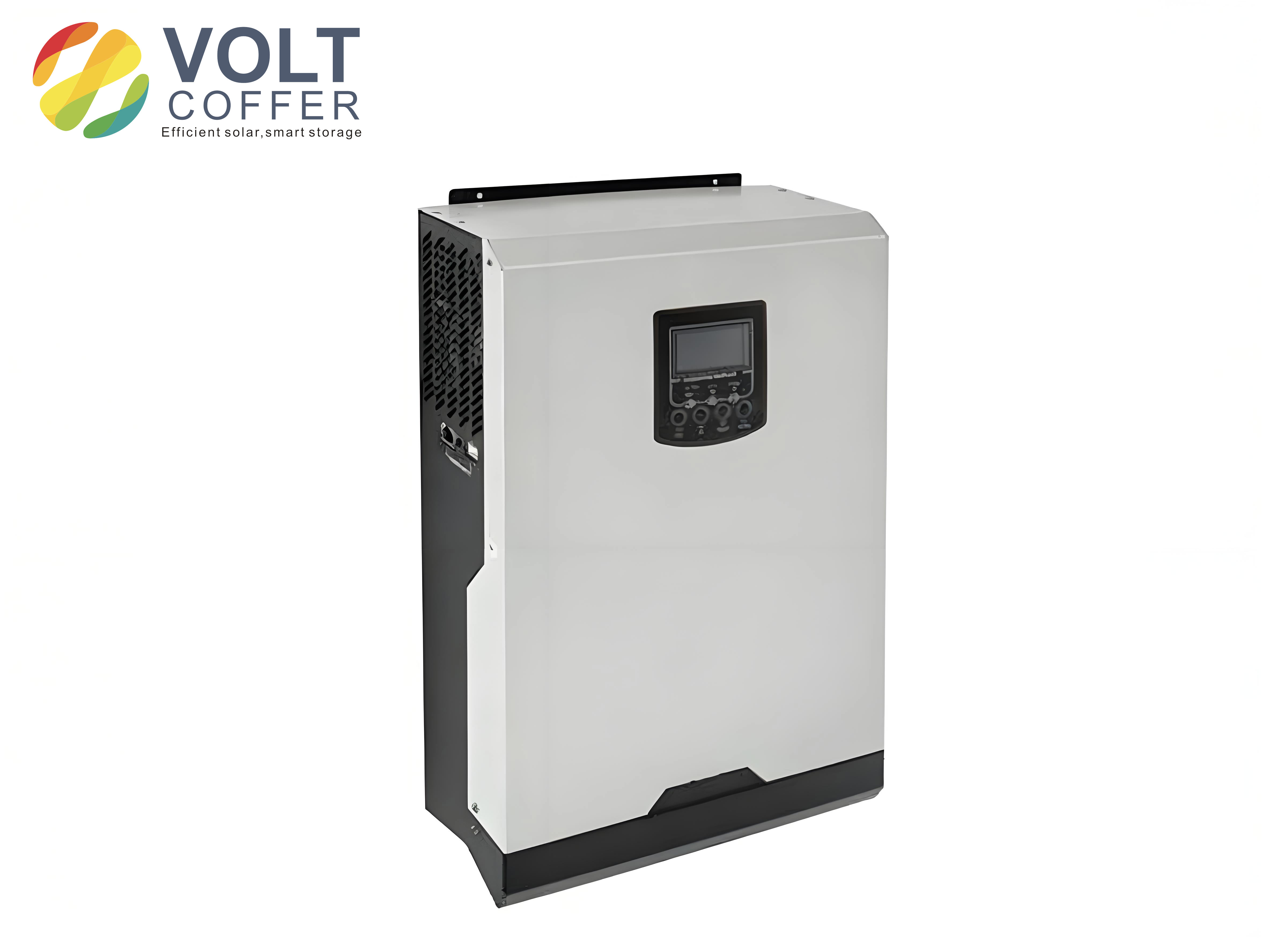
Energy Context and the Role of Solar Inverters. I start from the observation that energy shortage and environmental pollution have made renewable generation a strategic priority. Solar energy is widely distributed, abundant, and technically mature, but its output is direct current, while most loads and grids require alternating current. Therefore, solar inverters are the key interface between photovoltaic modules and the AC side. In a conventional centralized architecture, many panels are connected in series and parallel and then fed to one large inverter. This reduces cost per watt, but it also creates a single-point failure risk and makes maximum power point tracking less effective when panels are mismatched. String solar inverters improve this by giving each string its own converter, but they still cannot isolate the behavior of every panel. Micro solar inverters solve this by assigning one converter to one panel or to a very small group of panels. In my design work, I treat the micro solar inverter as a modular power electronics building block that can perform DC-DC boosting, maximum power point tracking, and DC-AC inversion.
The comparative advantage of GaN in solar inverters is rooted in material properties. Silicon has dominated power electronics for decades, but its bandgap, breakdown field, and thermal limits restrict further improvements in frequency and density. Silicon carbide offers higher voltage capability and good thermal performance, but GaN provides a strong combination of high electron mobility, high saturation velocity, and low switching charge. For low-voltage inputs such as a single photovoltaic module, this combination is particularly useful because the converter must boost a relatively low DC voltage to a high DC bus and then invert it to AC. In my simulations and prototype work, GaN devices enable higher switching frequency without proportional increases in switching loss, which is exactly what micro solar inverters need.
| Material | Bandgap (eV) | Electron mobility (cm²/V·s) | Breakdown field (MV/cm) | Thermal conductivity (W/cm·K) |
|---|---|---|---|---|
| Si | 1.12 | 1400 | 0.3 | 1.5 |
| GaAs | 1.42 | 8500 | 0.4 | 0.5 |
| SiC | 3.26 | 900 | 3.0 | 4.9 |
| GaN | 3.45 | 1500–2000 | 3.3 | 1.3 |
The intrinsic carrier concentration can be written as
$$n_i = \sqrt{N_C N_V} \exp\left(-\frac{E_g}{2kT}\right),$$
where \(E_g\) is the bandgap, \(k\) is Boltzmann’s constant, and \(T\) is absolute temperature. Because GaN has a much larger bandgap than silicon, its intrinsic carrier concentration is many orders of magnitude lower, which supports high-temperature operation and reduces leakage. For solar inverters, this means that GaN devices can maintain useful behavior under thermal stress and high electric field. I also note that the critical electric field of GaN is about ten times that of silicon, so a GaN device can achieve a given breakdown voltage with a much thinner and more heavily doped drift region. That lowers on-resistance and improves efficiency in solar inverters.
GaN HEMT Structure and Operating Principle. In my study, the core switching device is the GaN high-electron-mobility transistor. The AlGaN/GaN heterojunction forms a two-dimensional electron gas, or 2DEG, at the interface. This 2DEG is generated by spontaneous and piezoelectric polarization without intentional doping. The sheet carrier density can be approximated as
$$n_s = \frac{\sigma_{pol}}{q} – \frac{\epsilon}{q d}\left(q\phi_b + E_F – \Delta E_C\right),$$
where \(\sigma_{pol}\) is the polarization charge, \(\epsilon\) is the permittivity, \(d\) is the barrier thickness, \(\phi_b\) is the barrier height, \(E_F\) is the Fermi level, and \(\Delta E_C\) is the conduction-band offset. Because the 2DEG has high mobility and high saturation velocity, GaN HEMTs are well suited to high-frequency solar inverters. The first GaN transistors demonstrated in the 1990s were depletion-mode devices, but practical power converters require enhancement-mode behavior. In my design, I prefer enhancement-mode GaN HEMTs because they are normally off and can be driven with simpler and safer gate control than depletion-mode devices.
| Device type | Threshold behavior | Advantages | Limitations |
|---|---|---|---|
| Depletion-mode GaN HEMT | Normally on, \(V_{th}<0\) | Simple epitaxial structure; high mobility | Requires negative gate bias; complex fail-safe design |
| Enhancement-mode P-GaN HEMT | Normally off, \(V_{th}>0\) | Simple drive, low gate charge, fast switching | Gate reliability and threshold stability need care |
| Cascode GaN HEMT | Normally off through Si MOSFET | Robust threshold, familiar silicon gate drive | Higher package inductance; additional device in series |
For a P-GaN gate HEMT, the gate structure contains a p-type GaN cap and a metal contact. The gate behaves like a diode, so the gate-source voltage is clamped in a safe range. In my driver design, I must account for three different gate currents: a positive turn-on current, a negative turn-off current, and a steady-state current. These can be represented as
$$I_{on} = \frac{Q_g + C_{gs}V_{drive}}{t_{on}},$$
$$I_{off} = \frac{Q_g + C_{gs}V_{drive}}{t_{off}},$$
$$I_{ss} = \frac{V_{drive} – V_F}{R_{ss}},$$
where \(Q_g\) is gate charge, \(C_{gs}\) is gate-source capacitance, \(V_F\) is the forward voltage of the gate diode, and \(R_{ss}\) is the steady-state gate resistance. In my view, the gate drive is one of the most important differences between GaN-based solar inverters and silicon-based solar inverters. A poorly designed gate loop can produce ringing, false turn-on, or excessive loss, even if the GaN device itself is excellent.
Switching loss in a hard-switched converter can be approximated as
$$P_{sw} = \frac{1}{2}V_{DS}I_D(t_r+t_f)f_s + Q_gV_{GS}f_s + P_{oss},$$
where \(t_r\) and \(t_f\) are rise and fall times, \(f_s\) is switching frequency, and \(P_{oss}\) is output capacitance loss. Because GaN HEMTs have low \(Q_g\) and small output capacitance compared with silicon MOSFETs of similar voltage rating, the frequency-dependent part of \(P_{sw}\) is reduced. This is the main reason I select GaN for micro solar inverters. It allows the converter to operate at tens of kilohertz or even around one megahertz, which shrinks the transformer, inductor, and capacitor. In my simulation study, I compare 50 kHz and 1 MHz operation to show that the topology remains valid at high frequency while passive sizes and ripple behavior change.
Photovoltaic Cell Modeling. To design a solar inverter, I first need a reliable model of the photovoltaic source. A photovoltaic cell behaves like a current source in parallel with a diode, a shunt resistance, and a series resistance. The output current can be expressed as
$$I = I_{ph} – I_0\left[\exp\left(\frac{q(V+IR_s)}{AKT}\right)-1\right] – \frac{V+IR_s}{R_{sh}},$$
where \(I_{ph}\) is the photogenerated current, \(I_0\) is the reverse saturation current, \(q\) is electron charge, \(A\) is the diode ideality factor, \(K\) is Boltzmann’s constant, \(T\) is cell temperature, \(R_s\) is series resistance, and \(R_{sh}\) is shunt resistance. Because this equation is implicit, I use an engineering model for simulation:
$$I_L = I_{sc}\left[1 – B\left(\exp\left(\frac{V}{CU_{oc}}\right)-1\right)\right],$$
where \(I_{sc}\) is short-circuit current, \(U_{oc}\) is open-circuit voltage, and \(B\) and \(C\) are coefficients determined from the maximum power point. I calculate them as
$$B = \left(\frac{I_m}{I_{sc}}\right)\exp\left(-\frac{U_m}{CU_{oc}}\right),$$
$$C = \frac{U_m}{U_{oc}}\left[\ln\left(1-\frac{I_m}{I_{sc}}\right)\right]^{-1}.$$
For actual irradiance \(S\) and temperature \(T\), I apply corrections:
$$I_{sc,real} = I_{sc}\left[1+\alpha(T-T_{ref})\right]\frac{S}{S_{ref}},$$
$$I_{m,real} = I_m\left[1+\alpha(T-T_{ref})\right]\frac{S}{S_{ref}},$$
$$U_{oc,real} = U_{oc}\left[1-\gamma(T-T_{ref})\right]\left[1+\beta\ln\left(\frac{S}{S_{ref}}\right)\right],$$
$$U_{m,real} = U_m\left[1+\gamma(T-T_{ref})\right]\left[1+\beta\ln\left(\frac{S}{S_{ref}}\right)\right].$$
In my Simulink model, I use standard reference conditions \(S_{ref}=1000\ \text{W/m}^2\) and \(T_{ref}=25^\circ\text{C}\). The model produces the familiar single-peak power-voltage curve. When irradiance increases at constant temperature, short-circuit current rises strongly and open-circuit voltage rises slightly, so the maximum power increases. When temperature increases at constant irradiance, open-circuit voltage decreases, and the maximum power point moves to a lower voltage. These effects are important for solar inverters because they define the operating range of the DC-DC stage and the tracking window of the maximum power point tracker.
| Condition | Effect on \(I_{sc}\) | Effect on \(U_{oc}\) | Effect on \(P_{max}\) | Effect on \(V_{mpp}\) |
|---|---|---|---|---|
| Irradiance increases at constant temperature | Strong increase | Slight increase | Strong increase | Almost constant |
| Temperature increases at constant irradiance | Slight increase | Decrease | Decrease | Decrease |
| Partial shading | Complex, multiple steps | Complex | Multiple local maxima possible | Multiple local values |
Maximum Power Point Tracking for Solar Inverters. My solar inverter must extract as much energy as possible from the photovoltaic module. Since the maximum power point changes with irradiance and temperature, I study maximum power point tracking algorithms. The most common methods are constant voltage tracking, incremental conductance, and perturb and observe. Each has a different balance between speed, accuracy, and implementation complexity.
Constant voltage tracking uses the approximate relation
$$V_{ref} \approx k_{CV}U_{oc},$$
where \(k_{CV}\) is typically between 0.7 and 0.8. This method is simple and stable, but it is not truly adaptive. If irradiance changes, the true maximum power point voltage may move, so constant voltage tracking can lose efficiency. In my simulation, constant voltage tracking took about 0.45 s to settle after an irradiance step, which is slower than the other methods, although its steady-state oscillation was very small.
Incremental conductance is based on the condition that at the maximum power point,
$$\frac{dP}{dV}=0.$$
Because \(P=VI\), this becomes
$$\frac{dI}{dV} = -\frac{I}{V}.$$
If \(\frac{dI}{dV} > -\frac{I}{V}\), the operating point is to the left of the maximum power point, and the voltage should increase. If \(\frac{dI}{dV} < -\frac{I}{V}\), the operating point is to the right, and the voltage should decrease. In my simulation, incremental conductance reached the new maximum power point in about 0.05 s after an irradiance step. Its tracking speed and accuracy were good, but it showed some steady-state oscillation because of the fixed step size and numerical differentiation.
Perturb and observe, also called hill climbing, applies a small voltage perturbation and observes the resulting power change:
$$\Delta P = P(k)-P(k-1),$$
$$\Delta V = V(k)-V(k-1).$$
If \(\Delta P > 0\) and \(\Delta V > 0\), the voltage should continue increasing. If \(\Delta P > 0\) and \(\Delta V < 0\), the voltage should continue decreasing. If \(\Delta P < 0\), the perturbation direction should be reversed. In my simulation, perturb and observe also reached the new maximum power point in about 0.05 s. It is simple and widely used in industrial solar inverters, but it can oscillate around the maximum power point and may misjudge under rapidly changing irradiance.
| MPPT method | Key principle | Speed | Accuracy | Implementation cost | Main weakness |
|---|---|---|---|---|---|
| Constant voltage tracking | Hold voltage near a fixed fraction of \(U_{oc}\) | Slow | Moderate | Very low | Not adaptive to irradiance and temperature |
| Incremental conductance | Use \(\frac{dI}{dV}=-I/V\) | Fast | High | Moderate | Steady-state oscillation; sensitive to noise |
| Perturb and observe | Perturb voltage and observe power | Fast | High | Low | Oscillation; possible wrong direction under fast transients |
I also reviewed more advanced methods for solar inverters, including fuzzy logic control, particle swarm optimization, firefly algorithm, and neural-network-based tracking. These methods can improve global search under partial shading and can reduce steady-state oscillation. However, they require more computation and more careful tuning. For a micro solar inverter with a low-cost digital signal processor, I prefer a well-tuned incremental conductance or perturb-and-observe method with adaptive step size. This gives a good compromise between tracking speed and implementation burden.
Power Stage Topology Selection. In my design, I compare single-stage and two-stage architectures. A single-stage solar inverter combines boosting and inversion in one power stage. It can be compact and low cost, but the control is complex because the same switches must handle both energy transfer and output waveform synthesis. A two-stage architecture separates DC-DC conversion from DC-AC inversion. The first stage boosts the low photovoltaic voltage to a stable high DC bus, and the second stage converts the DC bus to AC. I choose a two-stage architecture because it simplifies control, improves modularity, and allows the DC bus to be regulated independently. This is particularly useful for micro solar inverters that must work over a wide input range.
| Architecture | Structure | Advantages | Disadvantages | Typical use |
|---|---|---|---|---|
| Single-stage solar inverter | One power conversion stage | Fewer components, compact | Complex control, limited optimization | Very low power |
| Two-stage solar inverter | DC-DC then DC-AC | Independent control, wide input range, easier MPPT | More components, higher cost | Micro and module-level solar inverters |
For the DC-DC stage, I analyze half-bridge, full-bridge, flyback, forward, push-pull, and push-pull forward topologies. The half-bridge has a simple structure, but the primary voltage is only half of the input, so voltage utilization is low. The full-bridge can handle high power, but it requires four switches and has shoot-through risk. The flyback is simple and low cost, but it stores energy in the transformer and is better for low-to-medium power with less stringent ripple requirements. The forward converter needs a reset winding and usually operates at low duty cycle. The push-pull converter has high voltage utilization, but it suffers from flux imbalance. The push-pull forward converter adds a clamping capacitor between the two primary windings, which suppresses flux imbalance and voltage spikes. For a low-voltage photovoltaic input and a high-voltage DC bus, I select the push-pull forward converter as the first stage of my solar inverter.
| DC-DC topology | Key features | Main limitation | Suitability for micro solar inverters |
|---|---|---|---|
| Half-bridge | Two switches, simple | Low voltage utilization | Medium |
| Full-bridge | Four switches, high power | Shoot-through, isolated drives | Low for low-voltage input |
| Flyback | Simple, low cost | Transformer energy storage, higher stress | Medium |
| Forward | Reset winding, low duty | Large transformer, low utilization | Medium |
| Push-pull | High utilization, two switches | Flux imbalance | High |
| Push-pull forward | Clamp capacitor suppresses imbalance and spikes | More careful transformer design | Very high |
For the DC-AC stage, I compare half-bridge and full-bridge inverters. The half-bridge uses two switches and two capacitors, but the DC bus utilization is lower and capacitor mismatch can cause imbalance. The full-bridge inverter uses four switches and can apply the full DC bus to the output filter in each half-cycle. It is more suitable for higher power and gives better voltage utilization. In my design, I select a full-bridge inverter for the second stage of the solar inverter. I use a bipolar sinusoidal pulse-width modulation method because it requires only two complementary high-frequency signals and is simpler to implement on a digital signal processor.
| DC-AC topology | Switches | Voltage utilization | Control complexity | Application |
|---|---|---|---|---|
| Half-bridge inverter | 2 | Lower | Moderate | Low-to-medium power |
| Full-bridge inverter | 4 | Higher | Higher | Medium-to-high power |
Operating Principle of the Push-Pull Forward Stage. In my selected first stage, the push-pull forward converter has two primary windings, two switches, one clamping capacitor, a transformer, a full-wave rectifier, and an LC filter. The clamping capacitor is connected between the two primary windings. When both switches are off, the input source, the two primary windings, and the clamping capacitor form a loop. This loop forces the magnetizing current to reset and reduces the voltage spike caused by leakage inductance. When one switch turns on, the input voltage is applied to one primary winding, and the clamping capacitor interacts with the other primary winding. The transformer secondary delivers energy to the rectifier and output filter. When the other switch turns on, the process is mirrored. The output voltage is approximately
$$V_o = 2nDV_{in},$$
where \(n=N_s/N_p\) is the turns ratio, \(D\) is the duty cycle of each switch, and \(V_{in}\) is the input voltage. I keep \(D\) below 0.45 to reserve dead time and avoid simultaneous conduction. The clamping capacitor value affects voltage stress and flux imbalance suppression. Its design equation can be written as
$$C = \frac{P_o(1-2D)T_s}{8V_{in}\Delta U_c},$$
where \(P_o\) is output power, \(T_s\) is switching period, and \(\Delta U_c\) is the allowed voltage ripple on the clamping capacitor. In my design, I choose a larger capacitor than the minimum calculated value to reduce voltage stress while still maintaining good flux balance. This is a key detail in GaN-based solar inverters because fast switching can excite leakage-inductance ringing, and the clamping capacitor helps damp that behavior.
Operating Principle of the Full-Bridge Inverter. The second stage is a full-bridge inverter with four GaN HEMTs. The two legs are driven with complementary SPWM signals. In bipolar modulation, when the modulation wave is positive and larger than the triangular carrier, the left leg applies positive bus voltage and the right leg applies negative bus voltage, so the load sees \(+V_{bus}\). When the modulation wave is smaller than the carrier, the output reverses to \(-V_{bus}\). The average output over a switching period follows the sinusoidal reference. The fundamental output can be approximated as
$$v_o(t) = m V_{bus}\sin(\omega t),$$
where \(m\) is the modulation index, \(V_{bus}\) is the DC bus voltage, and \(\omega=2\pi f_o\) is the angular output frequency. The output filter removes switching harmonics. For an LC filter, the cutoff frequency is
$$f_c = \frac{1}{2\pi\sqrt{LC}}.$$
I choose \(f_c\) between the fundamental frequency and one-tenth of the switching frequency. This ensures that the 50 Hz fundamental passes with little attenuation while the switching ripple is strongly suppressed. For solar inverters, the output filter must also handle the RMS current and must not introduce excessive reactive power or phase shift.
| Filter type | Order | Advantages | Disadvantages | Best use |
|---|---|---|---|---|
| L filter | First order | Simple, robust | Large inductance, poor high-frequency attenuation | Small power, high switching frequency |
| LC filter | Second order | Good high-frequency attenuation, faster dynamics | Not ideal for grid-tied operation without damping | Standalone and micro solar inverters |
| LCL filter | Third order | Excellent high-frequency attenuation | Resonance, complex control | Grid-connected solar inverters |
Control Strategy for the Two-Stage Solar Inverter. In my design, the first stage uses PWM closed-loop control. I sample the DC bus voltage, compare it with a reference, and feed the error into a PID controller. The output of the PID controller adjusts the duty cycle of the two push-pull forward switches. The control law can be written as
$$D(k) = K_p e(k) + K_i \sum_{j=0}^{k} e(j) + K_d\left[e(k)-e(k-1)\right],$$
where \(e(k)=V_{bus,ref}-V_{bus}(k)\). The duty cycle is limited to a safe maximum, typically 0.45 for each switch in my design. This prevents shoot-through and provides margin for transformer reset.
The second stage uses SPWM closed-loop control. I sample the output voltage, compare it with a sinusoidal reference, and use a PID controller to adjust the modulation index. The resulting SPWM signal drives the full-bridge switches. The reference is
$$v_{ref}(t) = V_m \sin(2\pi f_o t),$$
where \(V_m\) is the desired peak output voltage and \(f_o=50\ \text{Hz}\). The modulation index is updated as
$$m(k) = K_p e_v(k) + K_i \sum_{j=0}^{k} e_v(j) + K_d\left[e_v(k)-e_v(k-1)\right],$$
where \(e_v(k)=v_{ref}(k)-v_o(k)\). The modulation index is limited to avoid overmodulation and to keep total harmonic distortion low. In my simulations, this control structure produced stable DC bus voltage and a clean sinusoidal output.
Simulation Study. I built a complete Simulink model of the two-stage GaN-based micro solar inverter. The first stage uses the push-pull forward topology, and the second stage uses the full-bridge inverter. I tested both a 50 kHz switching frequency and a 1 MHz switching frequency. The DC input was 20 V. In the 50 kHz case, the first stage reached a stable DC bus of about 376 V, and the second stage produced a 308.8 V peak, 50 Hz sinusoidal output. The total harmonic distortion was 1.74 %, which is below the 5 % design target. In the 1 MHz case, the first stage reached about 374.5 V, and the second stage produced a 310.9 V peak, 50 Hz sinusoidal output. The total harmonic distortion was 1.37 %. These results confirm that the proposed two-stage solar inverter can operate at both conventional and high switching frequencies.
| Parameter | 50 kHz simulation | 1 MHz simulation |
|---|---|---|
| DC input | 20 V | 20 V |
| First-stage DC bus | Approximately 376 V | Approximately 374.5 V |
| Second-stage AC peak | Approximately 308.8 V | Approximately 310.9 V |
| Output frequency | 50 Hz | 50 Hz |
| THD | 1.74 % | 1.37 % |
| Control | PWM + SPWM closed loop | PWM + SPWM closed loop |
I also examined the drive waveforms. The first-stage PWM signals were complementary with a dead time, and the duty cycle was limited to 0.45. The second-stage SPWM signals were complementary and had a sinusoidally varying duty cycle. In the 1 MHz case, the pulse widths changed more slowly relative to the carrier period, but the sinusoidal modulation was still clearly visible over a longer time window. The DC bus showed small low-frequency ripple when the inverter stage was connected, because the AC load draws pulsating power. This ripple can be reduced by increasing the DC bus capacitor or by improving the control bandwidth, but in my design the bus remained stable enough for the second stage to produce a good sine wave.
Hardware Design of the Micro Solar Inverter. My hardware design is divided into four modules: the main power circuit, the auxiliary power supply, the gate drive circuit, and the sensing circuit. The main power circuit contains the push-pull forward DC-DC stage and the full-bridge DC-AC stage. The auxiliary power supply provides 12 V, 8 V, 5 V, 3.3 V, 1.65 V, and -12 V rails for the control, sensing, and gate drive circuits. The gate drive circuit uses an isolated GaN-specific driver. The sensing circuit measures photovoltaic voltage, DC bus voltage, output voltage, input current, and output current for closed-loop control and protection.
| Parameter | Design value |
|---|---|
| Input voltage | 20 VDC to 40 VDC |
| Output voltage | 220 VAC ± 5 % |
| Output frequency | 50 Hz ± 5 % |
| Rated output power | 200 W |
| Switching frequency | 50 kHz |
| Duty cycle limit | 0.45 |
| Efficiency target | 85 % to 90 % |
| THD target | Less than 5 % |
Transformer Design. The transformer is the most important magnetic component in the first stage. I selected a ferrite PQ4040 core because it provides a good balance between window area and effective cross-sectional area. The power capacity product is
$$SQ = \frac{T_{on}P_o}{\eta B_m K_w K_c j}\times 10^8,$$
where \(T_{on}\) is the on-time, \(P_o\) is output power, \(\eta\) is efficiency, \(B_m\) is maximum flux density, \(K_w\) is window utilization, \(K_c\) is core stacking factor, and \(j\) is current density. The turns ratio is
$$n = \frac{N_s}{N_p} = \frac{U_o + U_d + U_{Lf}}{D_m U_{in}},$$
where \(U_d\) is rectifier voltage drop and \(U_{Lf}\) is filter inductor voltage drop. I calculated a turns ratio of about 22. The primary turns are
$$N_p = \frac{U_{in}T_{on}}{2B_m A_e}\times 10^8,$$
and the secondary turns are \(N_s=nN_p\). I chose 3 primary turns and 66 secondary turns. For the primary winding, I used four strands of AWG23 wire in parallel. For the secondary winding, I used a single AWG26 wire. The skin depth is
$$H = \sqrt{\frac{2}{\omega \mu \gamma}},$$
where \(\omega=2\pi f_s\), \(\mu\) is permeability, and \(\gamma\) is conductivity. At 50 kHz, the skin depth in copper is about 0.296 mm, so the wire diameter should be less than about 0.592 mm. My selected wires satisfy this condition.
| Transformer parameter | Value |
|---|---|
| Core | PQ4040 ferrite |
| Effective area \(A_e\) | 2.010 cm² |
| Window area \(A_w\) | 3.260 cm² |
| Maximum flux density | 1700 Gs |
| Turns ratio | 22 |
| Primary turns | 3 |
| Secondary turns | 66 |
| Primary wire | 4 × AWG23 |
| Secondary wire | 1 × AWG26 |
| Window utilization | 0.036 |
Switch and Rectifier Selection. For the first stage, the switches must withstand at least twice the input voltage plus margin for leakage-inductance spikes. Since the input can reach 40 V, the switch voltage rating should be above 160 V after margin. The peak current is about 6.23 A, so a 10 A or higher current rating is appropriate. I selected a 600 V enhancement-mode GaN HEMT with 70 mΩ on-resistance and 60 A pulsed current capability. This provides large margin and low conduction loss. For the rectifier, I selected fast-recovery diodes with 600 V reverse voltage and 8 A forward current. Fast recovery is important because the rectifier operates at the switching frequency and reverse recovery loss would otherwise reduce efficiency.
| Component | Selected rating | Reason |
|---|---|---|
| First-stage GaN HEMT | 600 V, 31 A, 70 mΩ | High margin, low \(R_{DS(on)}\), fast switching |
| Second-stage GaN HEMT | 600 V, 31 A, 70 mΩ | Full-bridge bus voltage stress with margin |
| Rectifier diode | 600 V, 8 A, 12 ns recovery | Fast recovery for high-frequency rectification |
| Clamping capacitor | 15 μF | Reduces voltage stress and flux imbalance |
Output Filter Design. For the first-stage LC filter, I calculated the inductor for boundary conduction mode as
$$L_1 = \frac{U_{o1}(1-2D)T_s}{2\Delta I}.$$
The capacitor was estimated from the allowed output voltage ripple as
$$C_1 = \frac{U_{o1}(1-2D)}{32f_s^2L_1\Delta U_{o1}}.$$
After simulation and practical adjustment, I used a 3 mH inductor and a 220 μF / 450 V capacitor for the first-stage filter. For the second-stage LC filter, I designed the cutoff frequency around 2 kHz. The inductor and capacitor values follow
$$L_2 = \frac{U_o^2}{P_o f_c},$$
$$C_2 = \frac{1}{(2\pi f_c)^2 L_2}.$$
I selected a 10 mH output inductor and a 4 μF output capacitor. The inductor was wound on an iron-silicon-aluminum toroidal core with 135 turns of 1.4 mm enameled wire. This filter suppresses the switching harmonics and produces a smooth sinusoidal output. In my view, the output filter is a critical part of micro solar inverters because it determines both waveform quality and reactive power behavior.
| Filter stage | Component | Value | Purpose |
|---|---|---|---|
| First-stage DC filter | Inductor | 3 mH | Smooth rectified DC current |
| First-stage DC filter | Capacitor | 220 μF / 450 V | Reduce DC bus ripple |
| Second-stage AC filter | Inductor | 10 mH | Attenuate switching harmonics |
| Second-stage AC filter | Capacitor | 4 μF | Form low-pass LC network |
Gate Drive Design. The gate drive must provide positive turn-on voltage and negative turn-off voltage for the GaN HEMTs. I used an isolated GaN-specific driver with separate source and gate return paths. The driver includes a gate resistor network, a capacitor, and a Schottky diode for fast turn-off. The gate loop is kept short to reduce parasitic inductance. In my layout, the gate drive loop area is minimized, and the source Kelvin connection is used to reduce common-source inductance. This is essential for GaN-based solar inverters because high \(dv/dt\) and \(di/dt\) can cause false turn-on and ringing if the gate loop is not carefully designed.
The gate drive current can be approximated by
$$I_G = \frac{V_{drive}}{R_G + R_{internal}},$$
and the gate power loss is
$$P_G = Q_g V_{drive} f_s.$$
Because GaN HEMTs have low gate charge, the gate drive loss is lower than that of comparable silicon MOSFETs. This is especially beneficial in high-frequency solar inverters, where gate drive loss can become a significant part of total loss.
Digital Control Implementation. I implemented the digital control on a TMS320F28335 digital signal processor. The main program initializes the system, reads the analog-to-digital converter results, checks the input voltage range, and enables the PWM and SPWM modules. The first-stage PWM subroutine configures the ePWM module to produce two complementary signals with dead time. The second-stage SPWM subroutine uses a sine lookup table and updates the duty cycle according to the output voltage error. The sampling subroutine uses timer-triggered conversion channels for photovoltaic voltage, DC bus voltage, output voltage, input current, and output current.
| Software module | Function | Key hardware resource |
|---|---|---|
| Main program | Initialization, fault checking, loop scheduling | CPU, timers, GPIO |
| ADC sampling | Read \(V_{pv}\), \(V_{bus}\), \(V_o\), \(I_{in}\), \(I_o\) | ADC channels, timer trigger |
| PWM subroutine | Generate complementary PWM with dead time | ePWM module |
| SPWM subroutine | Generate sinusoidal PWM for full bridge | ePWM module, sine table |
| PID controller | Regulate DC bus and AC output | CPU, floating-point unit |
Auxiliary Power and Sensing. The auxiliary power supply is based on a wide-input buck regulator that accepts the photovoltaic voltage and generates the required positive rails. A separate isolated module generates -12 V for analog signal conditioning. The sensing circuits use resistor dividers for voltage, shunt and Hall-effect sensors for current, and operational amplifiers for level shifting and filtering. The analog signals are clamped to the 0 V to 3.3 V range before entering the DSP. This protects the controller and ensures accurate sampling. In my design, the photovoltaic voltage is divided down, the DC bus voltage is scaled through a differential amplifier, and the AC output voltage is biased around 1.65 V so that both positive and negative half-cycles can be measured.
| Sensing signal | Method | Purpose |
|---|---|---|
| Photovoltaic voltage | Resistor divider with clamping diodes | Input range check and MPPT |
| DC bus voltage | Divider, differential amplifier, RC filter | First-stage closed-loop regulation |
| Output voltage | Divider with 1.65 V bias | Second-stage closed-loop regulation |
| Input current | Shunt resistor and amplifier | Input power calculation and protection |
| Output current | Hall-effect sensor | Output power and overcurrent protection |
PCB Layout and Prototype. I designed the printed circuit boards in a modular way. The power board carries the main current path, the transformer, the GaN HEMTs, the rectifiers, and the output filters. The auxiliary power board generates the control rails. The sensing board contains the voltage and current conditioning circuits. In the power board layout, I kept the high-current loops short and wide, placed the decoupling capacitors close to the GaN devices, and separated the gate loop from the power loop. I also used thermal relief and copper pours to improve heat spreading. The prototype was assembled and tested with a programmable DC source, an oscilloscope, an electronic load, and a power resistor load.
| Prototype module | Function | Key design consideration |
|---|---|---|
| Power board | Push-pull forward and full-bridge power stage | Short high-current loops, thermal spreading |
| Control board | DSP and digital PWM generation | Clean clock, stable 3.3 V supply |
| Sensing board | Voltage and current measurement | Noise filtering and clamping |
| Auxiliary power board | 12 V, 8 V, 5 V, 3.3 V, 1.65 V, -12 V | Isolation and low ripple |
| Filter board | DC and AC filtering | Low ESR, low core loss |
Experimental Results. I first tested the auxiliary power supply. The measured 3.3 V rail was 3.332 V, and the measured 8 V rail was 7.903 V. These values are within the operating range of the driver and sensing circuits. I then tested the PWM waveform for the first stage. The two gate signals were complementary, with an amplitude of about 3.08 V before the driver and a frequency of 50 kHz. The duty cycle was about 0.45, and the dead time was visible. The SPWM waveform for the second stage had an amplitude of about 3.23 V and a duty cycle that varied sinusoidally. After the gate driver, the measured gate waveform had a peak-to-peak amplitude of about 4.68 V. The falling edge showed a negative pulse for reliable turn-off, which is important for the P-GaN HEMT. The output AC waveform was close to a sine wave with a frequency of about 50.75 Hz and an amplitude between about 292 V and 324 V. I observed some harmonics near the peak and zero crossing, likely caused by nonideal gate rise time, parasitic layout inductance, modular wiring, and nonoptimal filter tuning. Even so, the prototype verified the basic operation of the two-stage GaN-based micro solar inverter.
| Test item | Measured result | Observation |
|---|---|---|
| 3.3 V auxiliary rail | 3.332 V | Within tolerance |
| 8 V auxiliary rail | 7.903 V | Suitable for gate driver |
| PWM amplitude | 3.08 V | DSP output before driver |
| PWM frequency | 50 kHz | Complementary with dead time |
| PWM duty cycle | 0.45 | Within safe limit |
| SPWM amplitude | 3.23 V | Varying duty cycle |
| Gate waveform peak-to-peak | 4.68 V | Negative turn-off pulse observed |
| Output frequency | 50.75 Hz | Close to 50 Hz target |
| Output amplitude | 292 V to 324 V | Some harmonic distortion |
Discussion. My results show that GaN devices can be successfully applied to micro solar inverters. The push-pull forward stage provides high voltage utilization and suppresses flux imbalance, while the full-bridge stage provides good DC bus utilization and a clean sinusoidal output. The use of GaN HEMTs allows the converter to operate at high frequency, which reduces magnetic component size and improves power density. The main challenges I encountered were gate drive design, layout parasitics, and output filter tuning. GaN devices switch very fast, so parasitic inductance in the gate loop and power loop can cause ringing and electromagnetic interference. In future versions of my solar inverters, I would use a more compact layout, an integrated gate driver, and a carefully designed snubber or soft-switching technique to reduce ringing and improve efficiency.
Further Work. I see several directions for improving GaN-based micro solar inverters. First, I would add protection circuits for overvoltage, overcurrent, overtemperature, and anti-islanding. Second, I would explore soft-switching topologies such as active clamp and resonant converters to reduce switching loss further. Third, I would improve the maximum power point tracking algorithm with adaptive step size or a hybrid global search method to handle partial shading more effectively. Fourth, I would design a compact integrated magnetic component and a more integrated power module to reduce volume and parasitic inductance. Fifth, I would add communication and monitoring functions so that multiple micro solar inverters can be coordinated and monitored in a distributed photovoltaic system. Finally, I would test the system under grid-connected conditions and evaluate power quality, islanding detection, and compliance with grid codes.
| Future improvement | Expected benefit | Technical challenge |
|---|---|---|
| Protection and fault handling | Safer and more reliable solar inverters | Fast detection and coordination |
| Soft switching | Lower switching loss | Timing and control complexity |
| Adaptive or hybrid MPPT | Better energy harvest under partial shading | More computation and tuning |
| Integrated magnetics | Smaller volume and lower parasitics | Thermal and winding design |
| Communication and monitoring | Improved system-level management | Cost and protocol compatibility |
| Grid-connected operation | Direct utility interaction | Standards, synchronization, islanding |
In conclusion, I have studied, designed, simulated, and tested a GaN-based two-stage micro solar inverter. The first stage uses a push-pull forward DC-DC converter, and the second stage uses a full-bridge DC-AC inverter. The control system uses PWM and SPWM closed-loop regulation implemented on a digital signal processor. My simulation results show stable DC bus voltage and sinusoidal AC output at both 50 kHz and 1 MHz. The hardware prototype validates the auxiliary power, gate drive, PWM, SPWM, and output stages. Although the prototype still has room for improvement in output quality and layout optimization, the work confirms that GaN technology is a strong candidate for high-frequency, high-density micro solar inverters. I believe that continued development of GaN-based solar inverters will contribute to more efficient, more flexible, and more widely deployed photovoltaic energy systems.