
In the context of global energy transition, solar energy plays a pivotal role. Solar panels, as the core components of photovoltaic power generation systems, directly influence power generation efficiency and safety. However, during production, transportation, installation, and operation, solar panels are inevitably subject to foreign objects (such as bird droppings, dust, snow) and various defects (cracks, hot spots, electrical damage). Even a small amount of dust accumulation can reduce the power generation efficiency of solar panels by 10% to 20%, while defects like cracks and hot spots may pose safety risks, including fire hazards. Therefore, efficient and accurate detection of foreign objects and defects on solar panels is crucial for maintaining stable operation of photovoltaic power stations.
Traditional methods, such as HSV-based K-means clustering or SimAM-Ada YOLOv5, have limitations in handling complex backgrounds and small targets. Deep learning-based methods like YOLOv4-Tiny with attention mechanisms or YOLOv8 with VanillaNet improvements have shown promise, but they often suffer from high computational resource demands and insufficient feature extraction for diverse morphologies and textures. The latest YOLOv11n offers a lightweight architecture, but its performance in specific photovoltaic panel detection tasks remains suboptimal. To address these challenges, we propose FESI-YOLOv11n, an improved algorithm based on YOLOv11n, incorporating four key enhancements: C3k2_Faster_EMA module, SEAttention mechanism, a reconstructed detection head (Detect_Efficient), and Inner_DIoU loss function.
Here is an illustration of a solar panel array under inspection, highlighting the practical application scenario of our study:
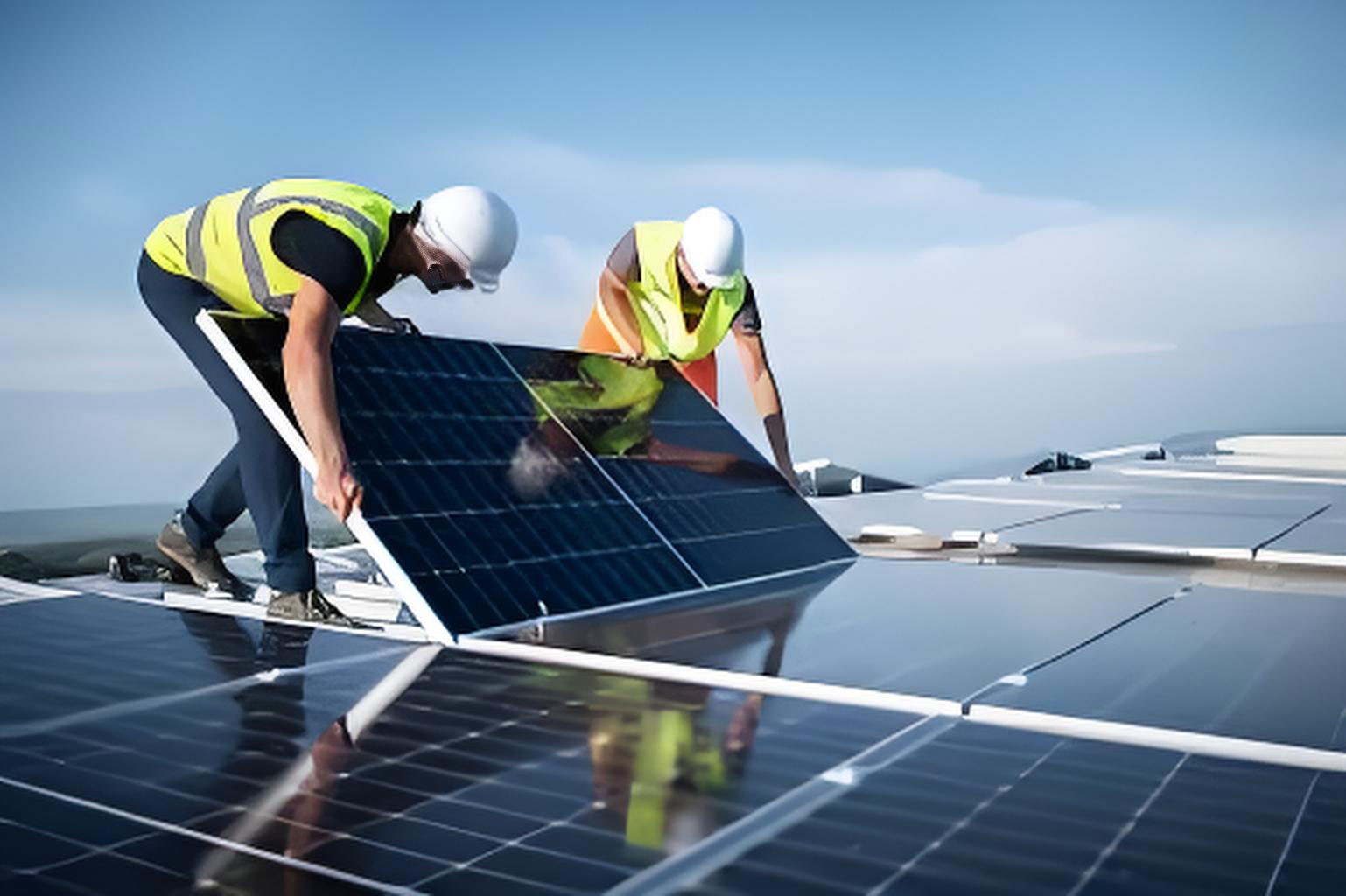
The proposed algorithm significantly improves detection accuracy while reducing model parameters and computational load, making it highly suitable for real-time monitoring of solar panels.
1. Background and Motivation
Photovoltaic (PV) power generation is a key technology for achieving carbon peak and carbon neutrality goals. Solar panels must operate under harsh outdoor conditions, exposing them to bird droppings, dust accumulation, snow cover, and various defects. Manual inspection is labor-intensive and inefficient. Existing automatic inspection methods often rely on traditional computer vision or shallow neural networks, which lack robustness. Deep learning-based object detection, especially the YOLO series, has demonstrated excellent speed and accuracy. However, YOLOv11n, despite its light weight, still suffers from low detection precision for small foreign objects and subtle defects on solar panels, as well as high computational overhead when applied to high-resolution imagery. Our goal is to enhance YOLOv11n to achieve higher precision, lower parameters, and faster inference for solar panel inspection.
2. Proposed Method: FESI-YOLOv11n
We introduce four major improvements to the original YOLOv11n architecture.
2.1 C3k2_Faster_EMA Module
The C3k2_Faster_EMA module replaces the standard C3k2 module in both the Backbone and Neck. It combines the Faster_Block_EMA structure with the C3k2 design. The Faster_Block uses partial convolution (PConv) to reduce computational redundancy: only a fraction of input channels undergo spatial convolution, while the rest are left unchanged. This reduces FLOPs by approximately 16 times compared to regular convolution and memory access by 4 times. The EMA (Efficient Multi-Scale Attention) mechanism groups channels and applies global average pooling and convolution to capture both global and local features, reweighting channels efficiently. By integrating these, the C3k2_Faster_EMA module achieves multi-scale feature extraction with lower parameters and computation. The bottleneck in the module uses two 3×3 convolutions instead of the original 1×3 and 3×3, approximating a 5×5 receptive field for stronger residual feature extraction – critical for capturing fine textures of solar panel defects.
The structure can be summarized as follows:
Input → CBS (Conv+BN+SiLU) → Split into two branches: one passes through C3_Faster_EMA (which contains N Bottleneck blocks) and the other is a shortcut. The outputs are concatenated and passed through another CBS.
Let the input tensor be $$X \in \mathbb{R}^{C \times H \times W}$$. The Partial Convolution (PConv) in FasterBlock is defined as:
$$ \text{PConv}(X) = [\text{Conv}_{k \times k}(X_{1:\alpha C}), X_{\alpha C+1:C}] $$
where $$\alpha$$ is the ratio of channels processed, typically $$\alpha=1/4$$. The remaining $1-\alpha$ channels are unchanged, reducing FLOPs. Subsequent 1×1 convolutions adjust dimensions.
Comparative experiments with other convolution modules (C3k2-RVB, iRMB-Cascaded, etc.) on our solar panel dataset show that Faster-EMA achieves the best balance of accuracy and efficiency, as shown in Table 1.
| Module | mAP50 (%) | mAP50-95 (%) | Parameters | GFLOPs |
|---|---|---|---|---|
| YOLOv11n (baseline) | 68.0 | 65.7 | 2,583,322 | 6.3 |
| +C3k2-RVB | 66.3 | 62.3 | 2,289,650 | 5.9 |
| +iRMB-Cascaded | 67.4 | 63.7 | 2,445,242 | 6.3 |
| +ContextGuided | 69.2 | 66.2 | 2,188,355 | 5.6 |
| +RFAConv | 69.5 | 66.9 | 2,636,786 | 6.6 |
| +C3k2-DRB | 70.1 | 67.5 | 2,443,410 | 6.3 |
| +Faster-EMA | 70.4 | 68.1 | 2,301,746 | 6.0 |
The C3k2_Faster_EMA module improves mAP50 by 2.4% and mAP50-95 by 2.4% over the baseline YOLOv11n, while reducing parameters by 10.9% and GFLOPs by 4.8%.
2.2 SEAttention Mechanism
To further enhance feature representation, we insert the SEAttention block after the C2PSA module in the Backbone. SEAttention (Squeeze-and-Excitation) learns channel-wise importance weights. It first performs global average pooling (squeeze) to obtain a channel descriptor $$z \in \mathbb{R}^{C}$$, then passes through two fully connected layers (excitation) to produce weights $$s = \sigma(W_2 \cdot \delta(W_1 z))$$, where $$\delta$$ is ReLU and $$\sigma$$ is sigmoid. The output feature map is scaled by these weights: $$\tilde{X} = X \cdot s$$. This mechanism helps the model focus on discriminative channels for solar panel defects, especially those with low contrast or small size.
We compared SEAttention with other attention modules (AFGCAttention, MLCA, Dattention, etc.) on our improved model. Results are in Table 2.
| Attention Module | mAP50 (%) | mAP50-95 (%) | Parameters | GFLOPs |
|---|---|---|---|---|
| AFGCAttention | 69.9 | 67.3 | 2,359,752 | 5.9 |
| MLCA | 70.4 | 68.0 | 2,301,756 | 5.9 |
| Dattention | 70.5 | 67.8 | 2,560,578 | 6.1 |
| SegNext_Attention | 70.7 | 68.4 | 2,387,906 | 6.0 |
| CAFM | 70.8 | 67.9 | 2,639,531 | 6.2 |
| TripletAttention | 70.9 | 68.5 | 2,294,154 | 5.9 |
| SEAttention | 71.2 | 68.7 | 2,302,146 | 5.9 |
SEAttention yields the highest mAP50 (71.2%) and mAP50-95 (68.7%), with only a marginal increase in parameters. The improvement is especially notable for detecting small foreign objects like bird droppings on solar panels.
2.3 Reconstructed Detection Head (Detect_Efficient)
We redesign the detection head by incorporating multi-branch and multi-scale ideas with reparameterization, inspired by EfficientNet’s weighted BiFPN and efficient head design. The original YOLOv11n head uses a simple convolution stack. Our Detect_Efficient head first applies two 3×3 grouped convolutions (groups=2) to reduce computation, then separates into class prediction and box prediction branches. Each branch uses a standard convolution (3×3 for class, 3×3 for box) before concatenating the outputs. This design reduces the number of parameters and FLOPs while maintaining or improving accuracy. The head takes multi-scale features from the Neck (P3~P7) and fuses them using channel-wise attention (BiFPN style) before prediction. The formulas for group convolution are:
$$ \text{GroupConv}(X) = \bigoplus_{g=1}^{G} \text{Conv}(X_g) $$
where $$G=2$$, splitting input channels into two groups. This reduces parameters to $$1/G$$ of standard convolution.
Comparative experiments with other detection heads (v10Detect, Detect_RSCD, etc.) are shown in Table 3.
| Detection Head | mAP50 (%) | mAP50-95 (%) | Parameters | GFLOPs |
|---|---|---|---|---|
| v10Detect | 65.8 | 63.4 | 2,302,146 | 5.9 |
| Detect_RSCD | 69.4 | 66.5 | 2,551,657 | 6.2 |
| MultiSEAMHead | 70.8 | 68.1 | 4,314,306 | 5.6 |
| Detect_SEAM | 70.9 | 68.4 | 2,210,370 | 5.3 |
| Detect_Efficient | 71.1 | 68.5 | 2,033,218 | 4.7 |
Detect_Efficient reduces parameters by 11.7% and GFLOPs by 20.3% compared to the best rival head, while maintaining mAP50 at 71.1%.
2.4 Inner_DIoU Loss Function
We replace the default CIoU loss with Inner_DIoU to improve bounding box regression. The DIoU loss adds a penalty based on the normalized distance between predicted and ground truth box centers:
$$ L_{DIoU} = 1 – IoU + \frac{\rho^2(b,b^{gt})}{c^2} $$
where $$\rho(b,b^{gt})$$ is the Euclidean distance between centers and $$c$$ is the diagonal length of the smallest enclosing box covering both boxes. Inner_DIoU further introduces an auxiliary bounding box concept, defined as:
$$ \text{Inner\_DIoU} = IoU – \frac{d^2}{c^2} $$
with $$d = \sqrt{(x_p – x_t)^2 + (y_p – y_t)^2}$$ and $$c = \sqrt{(x_{\max}-x_{\min})^2 + (y_{\max}-y_{\min})^2}$$. The auxiliary box is generated by scaling the original box with a factor, helping faster convergence and better regression for small targets typical on solar panels.
We compared Inner_DIoU with other loss functions (focaler_GIoU, EIoU, etc.) while keeping other improvements fixed. Results in Table 4.
| Loss Function | mAP50 (%) | mAP50-95 (%) | Parameters | GFLOPs |
|---|---|---|---|---|
| focaler_GIoU | 68.9 | 66.1 | 2,033,218 | 4.7 |
| EIoU | 69.4 | 66.9 | 2,033,218 | 4.7 |
| focaler_DIoU | 70.3 | 67.9 | 2,033,218 | 4.7 |
| mpdIoU | 70.7 | 68.1 | 2,033,218 | 4.7 |
| SIoU | 70.8 | 68.4 | 2,033,218 | 4.7 |
| DIoU | 71.2 | 68.7 | 2,033,218 | 4.7 |
| Inner_DIoU | 71.6 | 69.1 | 2,033,218 | 4.7 |
Inner_DIoU achieves the highest mAP50 (71.6%) and mAP50-95 (69.1%), with no extra parameters or computation.
3. Experiments and Results
3.1 Dataset and Settings
We curated a dataset of 12,887 images of solar panels from public sources (Baidu AI Studio, OpenML, Roboflow). Images have a resolution of 640×640 pixels and include six classes: bird-drop, clean, dusty, snow-covered, electrical-damage, and physical-damage. The dataset was split into training (10,309), validation (1,289), and test (1,289) sets. All experiments were conducted on an NVIDIA GeForce RTX 4060 Ti GPU with PyTorch 2.3.0. Training hyperparameters: optimizer SGD, epochs 300, batch size 16, workers 4, default augmentation (mosaic, mixup, etc.). Evaluation metrics include mAP50, mAP50-95, parameters (in millions), and GFLOPs.
3.2 Ablation Study
To verify the contribution of each component, we conducted ablation experiments by incrementally adding modules to the YOLOv11n baseline. Results are summarized in Table 5.
| Baseline | C3k2_Faster_EMA | SEAttention | Detect_Efficient | Inner_DIoU | mAP50 (%) | mAP50-95 (%) | Parameters | GFLOPs |
|---|---|---|---|---|---|---|---|---|
| ✓ | — | — | — | — | 68.0 | 65.7 | 2,583,322 | 6.3 |
| ✓ | ✓ | — | — | — | 70.4 | 68.1 | 2,301,746 | 6.0 |
| ✓ | ✓ | ✓ | — | — | 71.2 | 68.7 | 2,302,146 | 5.9 |
| ✓ | ✓ | ✓ | ✓ | — | 71.1 | 68.5 | 2,033,218 | 4.7 |
| ✓ | ✓ | ✓ | ✓ | ✓ | 71.6 | 69.1 | 2,033,218 | 4.7 |
The final FESI-YOLOv11n achieves a 3.6% increase in mAP50 and a 3.4% increase in mAP50-95, while reducing parameters by 21.29% and GFLOPs by 25.4% compared to the original YOLOv11n. Each module contributes positively, with the C3k2_Faster_EMA providing the largest accuracy gain and the Detect_Efficient head offering the most significant reduction in complexity.
3.3 Comparison with State-of-the-Art Models
We compared our model with mainstream YOLO variants: YOLOv6n, YOLOv8n, YOLOv9s, YOLOv10n, and YOLOv11n. Results are shown in Table 6.
| Model | mAP50 (%) | mAP50-95 (%) | Parameters | GFLOPs |
|---|---|---|---|---|
| YOLOv6n | 69.3 | 67.1 | 4,155,618 | 11.5 |
| YOLOv8n | 70.9 | 68.4 | 2,685,538 | 6.9 |
| YOLOv9s | 71.5 | 69.0 | 21,362,066 | 84.1 |
| YOLOv10n | 67.2 | 63.0 | 2,696,756 | 8.2 |
| YOLOv11n | 68.0 | 65.7 | 2,583,322 | 6.3 |
| FESI-YOLOv11n (Ours) | 71.6 | 69.1 | 2,033,218 | 4.7 |
Our model outperforms all YOLO variants in mAP50 and mAP50-95 while having the fewest parameters and flops. For instance, compared to YOLOv9s (which has 21.4M parameters and 84.1 GFLOPs), ours uses only 2.0M parameters and 4.7 GFLOPs, yet achieves higher accuracy. This lightweight design is ideal for edge deployment in solar panel inspection drones or embedded cameras.
We also present per-class confidence comparisons (from detection examples) in Table 7, showing that our model consistently achieves higher confidence across all defect types, especially for physical damage (0.80 vs. 0.67 for YOLOv11n) and snow-covered (0.87 vs. 0.77).
| Defect Type | YOLOv8n | YOLOv9s | YOLOv10n | YOLOv11n | FESI-YOLOv11n |
|---|---|---|---|---|---|
| bird-drop | 0.71, 0.57 | 0.85, 0.81 | 0.70, 0.62 | 0.74, 0.67 | 0.87, 0.73 |
| clean | 0.95 | 0.93 | 0.98 | 0.92 | 0.95 |
| dusty | 0.97 | 0.98 | 0.99 | 0.94 | 0.99 |
| electrical-damage | 0.56 | 0.83 | 0.68 | 0.42 | 0.78 |
| physical-damage | 0.67 | 0.55 | 0.59 | 0.67 | 0.80 |
| snow-covered | 0.61 | 0.84 | 0.60 | 0.77 | 0.87 |
The improved convergence curves (not shown due to page constraints) also indicate that FESI-YOLOv11n achieves lower loss and higher mAP values from early epochs, demonstrating faster learning.
4. Conclusion and Future Work
We have proposed FESI-YOLOv11n, an improved detection model specifically designed for foreign objects and defects on solar panels. By replacing the C3k2 module with C3k2_Faster_EMA, embedding SEAttention after C2PSA, adopting a lightweight Detect_Efficient head, and using Inner_DIoU loss, the model achieves a 3.6% increase in mAP50 (from 68.0% to 71.6%) and a 3.4% increase in mAP50-95 (from 65.7% to 69.1%), while reducing parameters by 21.3% and computational cost by 25.4%. Extensive ablation and comparison experiments validate the effectiveness of each component. The model surpasses current mainstream YOLO variants in both accuracy and efficiency, making it highly suitable for real-time solar panel inspection in smart photovoltaic systems.
Future work will focus on adapting the algorithm to more challenging scenarios, such as low-light conditions, severe occlusions, and different solar panel materials. Additionally, we plan to explore knowledge distillation or model pruning to further compress the model for edge devices, and to extend the detection to include more defect types (e.g., PID effect, delamination) that degrade solar panel performance.