
In the realm of advanced energy storage systems, the li ion battery stands as a cornerstone technology, powering everything from portable electronics to electric vehicles. Accurate monitoring and management of these batteries are paramount for ensuring safety, longevity, and efficiency. Central to an effective Battery Management System (BMS) is the precise estimation of internal states, particularly the State of Charge (SOC), which cannot be measured directly. This necessitates the use of mathematical models that can faithfully represent the battery’s dynamic behavior. Equivalent circuit models (ECMs), composed of resistive and capacitive elements, have been widely adopted for this purpose due to their balance between complexity and physical interpretability. Traditional models, such as the integer-order Thevenin model, have served well but often face limitations in capturing the nuanced electrochemical processes within a li ion battery. Recently, fractional calculus has emerged as a powerful tool, leading to the development of fractional-order ECMs that incorporate Constant Phase Elements (CPE), offering a more accurate representation of the battery’s impedance spectrum. In this comprehensive study, we explore and compare the performance of three distinct circuit models—integer first-order, integer second-order, and fractional first-order—in estimating the SOC of a li ion battery. Our approach integrates online parameter identification using the Forgetting Factor Recursive Least Squares (FFRLS) method and state estimation via the Extended Kalman Filter (EKF). Through rigorous experimental validation under dynamic stress conditions, we demonstrate the superior accuracy of the fractional-order model, highlighting its potential for enhancing BMS capabilities. The following sections delve into the model formulations, identification techniques, estimation algorithms, and detailed results, supported by numerous equations and summary tables.
The performance and reliability of any li ion battery system hinge on the BMS’s ability to infer critical states like SOC. SOC is defined as the ratio of remaining charge to the battery’s maximum capacity, typically expressed as a percentage. Direct measurement of SOC is impractical; hence, model-based estimation techniques are employed. These techniques rely on an accurate mathematical representation of the battery’s terminal behavior. Equivalent circuit models are favored for their simplicity and real-time feasibility. They approximate the internal electrochemical processes using electrical components: voltage sources for open-circuit voltage (OCV), resistors for ohmic losses, and RC networks for polarization dynamics. However, the standard integer-order RC elements sometimes fail to fully capture the distributed time constants and frequency-dependent behavior observed in a real li ion battery. This is where fractional-order models, grounded in fractional calculus, offer a significant advancement. By replacing ideal capacitors with CPEs, which have impedance of the form $Z_{CPE} = 1/[C(j\omega)^{\alpha}]$, these models provide a more flexible and accurate fit to electrochemical impedance spectroscopy (EIS) data. The parameter $\alpha$, the fractional order, lies between -1 and 1 and allows for modeling phenomena like diffusion and charge transfer with greater fidelity. This study systematically evaluates whether this theoretical advantage translates to tangible improvements in SOC estimation accuracy compared to conventional integer-order models.
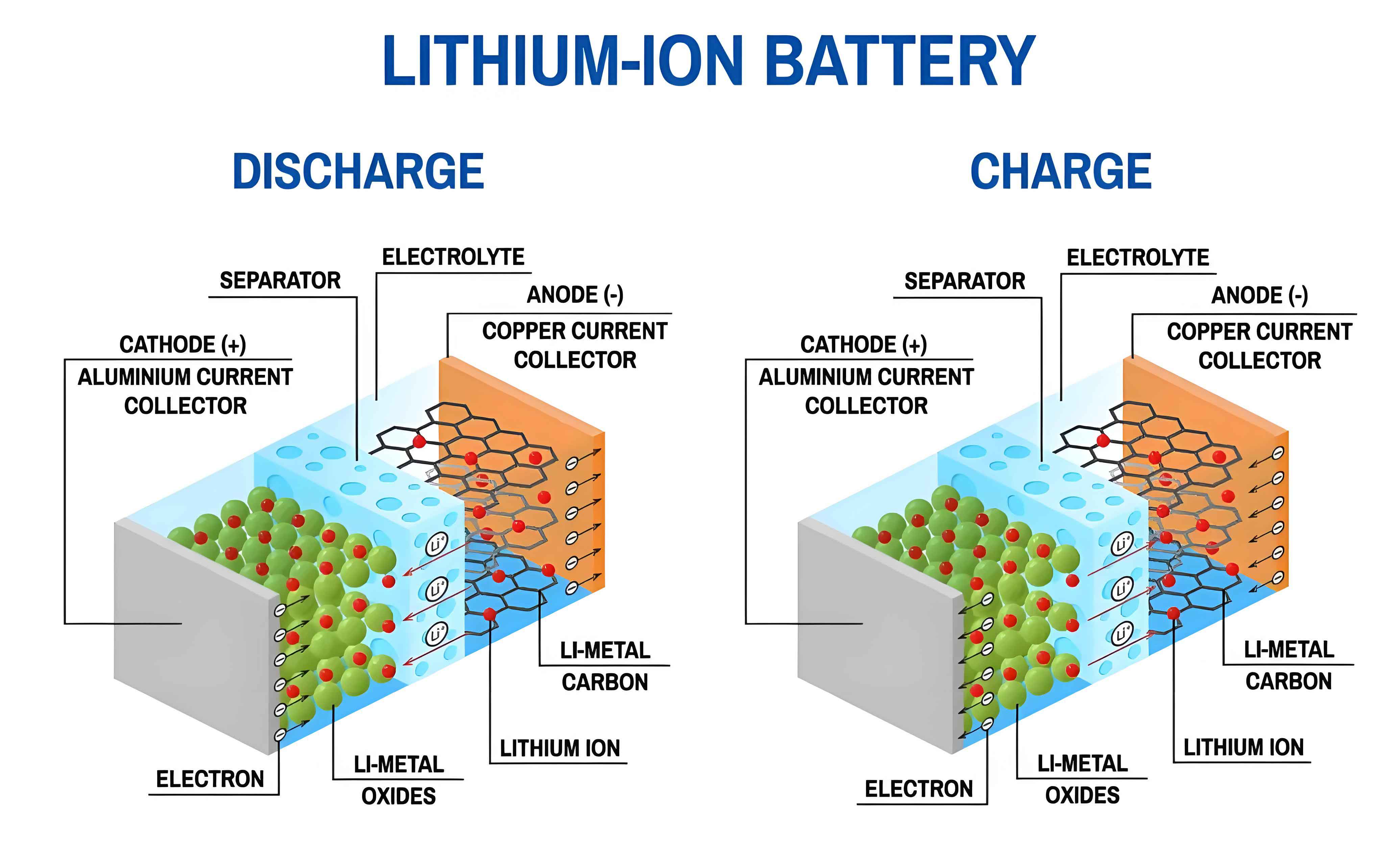
We begin by establishing the mathematical foundations of the three equivalent circuit models for the li ion battery. The first model is the integer first-order RC model, often referred to as the Thevenin model. It consists of an OCV source $U_{oc}$, an ohmic resistor $R_0$, and a single parallel RC branch ($R_1$, $C_1$) representing the dominant polarization effect. The governing equations in the continuous-time domain are:
$$ U_L(t) = U_{oc}(SOC(t)) – U_1(t) – I(t)R_0 $$
$$ C_1 \frac{dU_1(t)}{dt} = I(t) – \frac{U_1(t)}{R_1} $$
Here, $U_L$ is the terminal voltage, $I$ is the current (positive for discharge), and $U_1$ is the voltage across the polarization RC branch. The SOC is related to current through the coulomb counting principle:
$$ SOC(t) = SOC(t_0) – \frac{1}{Q_n} \int_{t_0}^{t} I(\tau) d\tau $$
where $Q_n$ is the nominal capacity of the li ion battery. For digital implementation in estimation algorithms, we discretize these equations. Using a sampling period $T$ and assuming zero-order hold for the current, the discrete-time state-space representation is derived:
$$
\begin{bmatrix}
SOC_{k+1} \\
U_{1,k+1}
\end{bmatrix}
=
\begin{bmatrix}
1 & 0 \\
0 & e^{-T/(R_1 C_1)}
\end{bmatrix}
\begin{bmatrix}
SOC_k \\
U_{1,k}
\end{bmatrix}
+
\begin{bmatrix}
-\frac{T}{Q_n} \\
R_1(1 – e^{-T/(R_1 C_1)})
\end{bmatrix}
I_k
$$
$$
U_{L,k} = \frac{\partial U_{oc}(SOC_k)}{\partial SOC_k} \cdot SOC_k – U_{1,k} – R_0 I_k
$$
This forms the basis for the EKF algorithm. The second model is the integer second-order RC model, which enhances the first-order model by adding another parallel RC branch ($R_2$, $C_2$) to account for a second polarization phenomenon, often associated with concentration polarization. This addition aims to improve the dynamic representation of the li ion battery. The continuous-time equations become:
$$ U_L(t) = U_{oc}(SOC(t)) – U_1(t) – U_2(t) – I(t)R_0 $$
$$ C_1 \frac{dU_1(t)}{dt} = I(t) – \frac{U_1(t)}{R_1} $$
$$ C_2 \frac{dU_2(t)}{dt} = I(t) – \frac{U_2(t)}{R_2} $$
The corresponding discrete-time state-space model, with states $[SOC, U_1, U_2]^T$, is:
$$
\begin{bmatrix}
SOC_{k+1} \\
U_{1,k+1} \\
U_{2,k+1}
\end{bmatrix}
=
\begin{bmatrix}
1 & 0 & 0 \\
0 & e^{-T/(R_1 C_1)} & 0 \\
0 & 0 & e^{-T/(R_2 C_2)}
\end{bmatrix}
\begin{bmatrix}
SOC_k \\
U_{1,k} \\
U_{2,k}
\end{bmatrix}
+
\begin{bmatrix}
-\frac{T}{Q_n} \\
R_1(1 – e^{-T/(R_1 C_1)}) \\
R_2(1 – e^{-T/(R_2 C_2)})
\end{bmatrix}
I_k
$$
$$
U_{L,k} = \frac{\partial U_{oc}(SOC_k)}{\partial SOC_k} \cdot SOC_k – U_{1,k} – U_{2,k} – R_0 I_k
$$
The third and most advanced model is the fractional first-order equivalent circuit model. In this configuration, the ideal capacitor $C_1$ in the polarization branch is replaced by a Constant Phase Element (CPE). The impedance of the CPE is given by $Z_1 = 1/[C_1 (j\omega)^{\alpha}]$, where $\alpha$ is the fractional order. This modification allows the model to better represent the distributed processes within the li ion battery. The continuous-time fractional differential equation for the polarization voltage is:
$$ C_1 \frac{d^{\alpha} U_1(t)}{dt^{\alpha}} = I(t) – \frac{U_1(t)}{R_1} $$
where $\frac{d^{\alpha}}{dt^{\alpha}}$ denotes the fractional derivative of order $\alpha$. To discretize this equation, we employ the Grünwald-Letnikov definition, which is suitable for numerical computation. The discrete approximation leads to the following state-space form:
$$
\begin{bmatrix}
SOC_{k+1} \\
U_{1,k+1}
\end{bmatrix}
=
\begin{bmatrix}
1 & 0 \\
0 & \frac{\alpha R_1 C_1}{T^{\alpha} + R_1 C_1}
\end{bmatrix}
\begin{bmatrix}
SOC_k \\
U_{1,k}
\end{bmatrix}
+
\begin{bmatrix}
-\frac{T}{Q_n} \\
\frac{T^{\alpha} R_1}{T^{\alpha} + R_1 C_1}
\end{bmatrix}
I_k
$$
$$
U_{L,k} = \frac{\partial U_{oc}(SOC_k)}{\partial SOC_k} \cdot SOC_k – U_{1,k} – R_0 I_k
$$
For simplicity and focus, the fractional order $\alpha$ is often fixed or identified offline; in our subsequent analysis, we assume a nominal value. A comparison of the model structures is summarized in Table 1.
| Model Type | Electrical Components | Key Parameters | Governing Dynamics |
|---|---|---|---|
| Integer First-Order | $U_{oc}$, $R_0$, $R_1$, $C_1$ | $R_0$, $R_1$, $C_1$ | Single exponential relaxation |
| Integer Second-Order | $U_{oc}$, $R_0$, $R_1$, $C_1$, $R_2$, $C_2$ | $R_0$, $R_1$, $C_1$, $R_2$, $C_2$ | Double exponential relaxation |
| Fractional First-Order | $U_{oc}$, $R_0$, $R_1$, CPE ($C_1$, $\alpha$) | $R_0$, $R_1$, $C_1$, $\alpha$ | Fractional-order relaxation |
The accuracy of any model-based estimator for a li ion battery is profoundly dependent on the precision of its parameters. These parameters are not constant; they vary with factors such as SOC, temperature, and aging. Therefore, online parameter identification is crucial for adaptive estimation. We employ the Forgetting Factor Recursive Least Squares (FFRLS) method, an enhancement of the standard RLS algorithm. The FFRLS introduces a forgetting factor $\lambda$ (typically $0.95 < \lambda \leq 1$) that discounts older data, allowing the algorithm to track time-varying parameters effectively, which is essential for a li ion battery under dynamic operating conditions.
The general form of a linear-in-parameters model is $y(k) = \boldsymbol{\varphi}^T(k) \boldsymbol{\theta}(k)$, where $y(k)$ is the observed output (e.g., terminal voltage error), $\boldsymbol{\varphi}(k)$ is the regression vector containing measured signals, and $\boldsymbol{\theta}(k)$ is the parameter vector to be identified. For the integer first-order model, by manipulating the discretized equations, we can express the terminal voltage as a linear function of parameters. A similar procedure is applied to the other models. The FFRLS algorithm proceeds iteratively as follows:
- Initialization: Set initial parameter estimate $\hat{\boldsymbol{\theta}}(0)$ and covariance matrix $\mathbf{P}(0)$ (often a large diagonal matrix). Choose forgetting factor $\lambda$.
- For each time step $k$:
- Compute the innovation (prediction error): $e(k) = y(k) – \boldsymbol{\varphi}^T(k) \hat{\boldsymbol{\theta}}(k-1)$.
- Calculate the gain vector: $\mathbf{K}(k) = \frac{\mathbf{P}(k-1) \boldsymbol{\varphi}(k)}{\lambda + \boldsymbol{\varphi}^T(k) \mathbf{P}(k-1) \boldsymbol{\varphi}(k)}$.
- Update the parameter estimate: $\hat{\boldsymbol{\theta}}(k) = \hat{\boldsymbol{\theta}}(k-1) + \mathbf{K}(k) e(k)$.
- Update the covariance matrix: $\mathbf{P}(k) = \frac{1}{\lambda} [\mathbf{I} – \mathbf{K}(k) \boldsymbol{\varphi}^T(k)] \mathbf{P}(k-1)$.
This recursive process continuously refines the parameter estimates as new data from the li ion battery becomes available. The regression vectors for the three models differ. For the integer first-order model, a common form is derived from the discrete transfer function relating terminal voltage to current. The parameters identified typically include $R_0$, $R_1$, and a time constant $\tau_1 = R_1C_1$. For the fractional-order model, the derivation is more involved due to the non-integer order; often, a fixed $\alpha$ is assumed, and $R_0$, $R_1$, and $C_1$ are identified. The FFRLS method’s ability to handle such variations makes it a robust choice for online adaptation in li ion battery management systems.
With a dynamically identified model, the next step is state estimation, specifically SOC estimation. The Extended Kalman Filter (EKF) is a prevalent nonlinear estimator that linearizes the system dynamics around the current state estimate. Given the nonlinear relationship between OCV and SOC ($U_{oc}(SOC)$), the EKF is well-suited for this task. The general nonlinear discrete-time system is represented as:
$$
\mathbf{x}_{k+1} = f(\mathbf{x}_k, \mathbf{u}_k) + \mathbf{w}_k
$$
$$
y_k = h(\mathbf{x}_k, \mathbf{u}_k) + v_k
$$
where $\mathbf{x}_k$ is the state vector (e.g., $[SOC_k, U_{1,k}]^T$ for the first-order model), $\mathbf{u}_k$ is the input (current $I_k$), $y_k$ is the output (terminal voltage $U_{L,k}$), and $\mathbf{w}_k$, $v_k$ are process and measurement noise, assumed to be zero-mean white Gaussian with covariances $\mathbf{Q}$ and $R$, respectively. The EKF algorithm consists of two main steps: prediction and update.
Prediction Step:
$$
\hat{\mathbf{x}}_{k|k-1} = f(\hat{\mathbf{x}}_{k-1|k-1}, \mathbf{u}_{k-1})
$$
$$
\mathbf{P}_{k|k-1} = \mathbf{A}_k \mathbf{P}_{k-1|k-1} \mathbf{A}_k^T + \mathbf{Q}
$$
Update Step:
$$
\tilde{y}_k = y_k – h(\hat{\mathbf{x}}_{k|k-1}, \mathbf{u}_k)
$$
$$
\mathbf{S}_k = \mathbf{C}_k \mathbf{P}_{k|k-1} \mathbf{C}_k^T + R
$$
$$
\mathbf{K}_k = \mathbf{P}_{k|k-1} \mathbf{C}_k^T \mathbf{S}_k^{-1}
$$
$$
\hat{\mathbf{x}}_{k|k} = \hat{\mathbf{x}}_{k|k-1} + \mathbf{K}_k \tilde{y}_k
$$
$$
\mathbf{P}_{k|k} = (\mathbf{I} – \mathbf{K}_k \mathbf{C}_k) \mathbf{P}_{k|k-1}
$$
Here, $\mathbf{A}_k$ and $\mathbf{C}_k$ are the Jacobian matrices of the functions $f$ and $h$ with respect to the state, evaluated at the prior estimate $\hat{\mathbf{x}}_{k-1|k-1}$:
$$ \mathbf{A}_k = \left. \frac{\partial f}{\partial \mathbf{x}} \right|_{\hat{\mathbf{x}}_{k-1|k-1}, \mathbf{u}_{k-1}}, \quad \mathbf{C}_k = \left. \frac{\partial h}{\partial \mathbf{x}} \right|_{\hat{\mathbf{x}}_{k|k-1}, \mathbf{u}_k} $$
For the integer first-order model, these Jacobians are straightforward to compute from the state-space equations. For the fractional-order model, the linearized matrices depend on the discretization method used. The OCV-SOC relationship, $U_{oc}(SOC)$, is a critical nonlinear function typically obtained through experimental characterization of the li ion battery. A common approach is to use a lookup table or a polynomial fit. The derivative $\frac{\partial U_{oc}(SOC)}{\partial SOC}$ is then used in the output matrix $\mathbf{C}_k$. The EKF, fueled by the online-identified parameters from FFRLS, provides a robust framework for real-time SOC estimation.
To validate and compare the three models, experimental tests were conducted on a commercial lithium iron phosphate (LiFePO4) li ion battery with a nominal capacity of 36 Ah. The battery was subjected to a Dynamic Stress Test (DST) profile, which includes varied charge and discharge pulses to simulate real-world usage. The current and terminal voltage were sampled at a fixed interval. The initial SOC was known, and reference SOC values were calculated using high-precision coulomb counting with periodic resets to ensure accuracy. The parameter identification and SOC estimation algorithms were implemented in a co-simulation environment.
The FFRLS algorithm was run online for each model. The forgetting factor $\lambda$ was set to 0.995 to balance tracking speed and stability. The identified parameters for the three models over the test cycle are summarized in Table 2. Note that parameters like $R_0$ show similar trends across models, while the polarization parameters differ. For the integer second-order model, the second RC branch parameters ($R_2$, $C_2$) are generally smaller than those of the first branch, indicating a faster dynamics component. For the fractional first-order model, the fractional order $\alpha$ was fixed at 0.5 based on preliminary EIS analysis of the li ion battery, and $C_1$ takes on a different numerical interpretation compared to the integer-order capacitance.
| Parameter | Integer First-Order | Integer Second-Order | Fractional First-Order ($\alpha=0.5$) |
|---|---|---|---|
| $R_0$ (mΩ) | 2.1 – 3.5 | 2.0 – 3.4 | 2.0 – 3.5 |
| $R_1$ (mΩ) | 1.5 – 4.0 | 1.8 – 5.0 | 1.6 – 4.2 |
| $C_1$ (kF or F*sα-1) | 8 – 15 | 6 – 12 | 5 – 10 (in fractional units) |
| $R_2$ (mΩ) | N/A | 0.8 – 2.5 | N/A |
| $C_2$ (kF) | N/A | 1 – 5 | N/A |
Using these identified parameters, the EKF was executed to estimate SOC. The process noise covariance $\mathbf{Q}$ and measurement noise covariance $R$ were tuned based on empirical data from the li ion battery. The terminal voltage predicted by each model (using the identified parameters and estimated states) was compared against the measured terminal voltage. The voltage prediction error, defined as $U_{L,meas} – U_{L,pred}$, is a direct indicator of model fidelity. The Root Mean Square Error (RMSE) and Maximum Absolute Error (MAE) for the voltage prediction across the entire test cycle were computed and are presented in Table 3.
| Model | RMSE (mV) | MAE (mV) |
|---|---|---|
| Integer First-Order | 24.5 | 58.3 |
| Integer Second-Order | 12.1 | 31.7 |
| Fractional First-Order | 8.7 | 22.4 |
The results clearly show that the fractional first-order model achieves the lowest voltage prediction errors, underscoring its superior ability to capture the terminal behavior of the li ion battery. The integer second-order model performs better than the first-order model but is outperformed by the fractional-order model. This is significant because the fractional model achieves this with a lower order (one fractional state versus two integer states), implying a more parsimonious representation of the underlying physics of the li ion battery.
The ultimate metric of performance is the accuracy of SOC estimation. The estimated SOC from each model’s EKF was compared against the reference SOC. The SOC estimation error, $SOC_{ref} – SOC_{est}$, was calculated throughout the discharge cycle. The statistical summary of these errors is provided in Table 4.
| Model | Mean Error (%) | RMSE (%) | Maximum Absolute Error (%) |
|---|---|---|---|
| Integer First-Order | -2.1 | 8.3 | 12.5 |
| Integer Second-Order | -0.8 | 6.9 | 10.2 |
| Fractional First-Order | 0.2 | 1.4 | 3.8 |
The data reveals a striking improvement offered by the fractional-order model. While the integer first-order model exhibits an SOC RMSE around 8%, and the integer second-order model reduces it to about 7%, the fractional first-order model achieves an RMSE of merely 1.4%. This represents a substantial enhancement in estimation accuracy for the li ion battery. The maximum error also follows the same trend, with the fractional model keeping errors within 4% throughout the dynamic test, whereas the integer models show deviations exceeding 10%. These findings robustly support the hypothesis that fractional-order dynamics provide a more truthful representation of the electrochemical processes in a li ion battery, leading to markedly better state observability.
The superior performance of the fractional first-order model can be attributed to its inherent ability to model memory and hereditary properties, which are characteristic of diffusion and charge transfer phenomena in a li ion battery. The CPE, with its power-law impedance, effectively captures the distributed time constants that a single or even two ideal RC branches can only approximate. This results in a model that requires fewer parameters than a high-order integer model to achieve comparable or better accuracy, reducing computational burden—a vital consideration for real-time BMS implementation. Furthermore, the online parameter identification via FFRLS ensures that the model adapts to changing conditions of the li ion battery, such as aging or temperature variations, maintaining estimation accuracy over time.
It is important to acknowledge the challenges associated with fractional-order models. The numerical computation of fractional derivatives is more complex than integer-order calculus, requiring careful discretization schemes like the Grünwald-Letnikov method. Additionally, the online identification of the fractional order $\alpha$ itself is a challenging nonlinear problem, often addressed offline or with sophisticated algorithms. In this study, we fixed $\alpha$ to simplify the online identification process; however, future work could involve joint estimation of $\alpha$ and other parameters for an even more adaptive model of the li ion battery.
In conclusion, this comprehensive investigation into equivalent circuit models for SOC estimation in li ion batteries demonstrates the clear advantages of incorporating fractional calculus. Through a structured comparison of integer first-order, integer second-order, and fractional first-order models, coupled with online FFRLS parameter identification and EKF-based state estimation, we have quantitatively shown that the fractional-order model achieves significantly higher accuracy in both terminal voltage prediction and SOC estimation. The fractional model’s RMSE for SOC was around 1%, outperforming the 7-8% errors of the integer models. This advancement is crucial for developing more reliable and efficient battery management systems, ultimately enhancing the performance and safety of applications reliant on li ion battery technology. As the demand for precise energy management grows, the adoption of fractional-order modeling represents a promising pathway toward unlocking the full potential of li ion batteries in modern energy storage systems.