
The efficiency of a solar photovoltaic (PV) system is intrinsically linked to the operating temperature of its cells. As the temperature of a PV module rises, its electrical conversion efficiency decreases significantly, typically in the range of -0.4% to -0.5% per degree Celsius for crystalline silicon cells. This thermal loss represents a major barrier to maximizing the energy yield from solar installations. A substantial portion of incident solar radiation, often exceeding 80%, is not converted into electricity but is instead dissipated as heat, elevating the module’s temperature and further depressing its performance. To address this fundamental challenge, effective cooling strategies for PV modules are essential. Among various passive and active cooling methods, front-surface water cooling presents a compelling dual-purpose solution: it actively reduces the cell temperature to boost electrical output while simultaneously cleaning the module surface of dust and debris, which can also cause performance losses. This article delves into the application characteristics of a solar system employing this front-surface water cooling technique, establishing a theoretical model, presenting experimental validation, and conducting a comparative analysis with a fixed-tilt, uncooled reference system.
Theoretical Heat Transfer Model for a Water-Cooled Solar System
The cooling mechanism involves a thin, flowing water film over the front glass surface of a standard PV module. The primary heat transfer modes for such a water-cooled solar system are forced convection on the front surface (water-film to glass) and natural convection combined with radiation on the rear surface (module backsheet to ambient). The energy balance for the PV module, treated as an object with a uniform temperature \(T\) (taken as the average of front and back surface temperatures), is governed by the following non-steady-state equation:
$$ C_{mod} \frac{dT}{dt} = A(1 – \rho)\tau I_s – Q_c – Q_r – P_{out} $$
where \( C_{mod} \) is the total heat capacity of the module (2918 J/K for the studied module), \(A\) is the module area (1.3 m²), \(\rho\) is the water film’s solar reflectance (~0.1), \(\tau\) is its transmittance (~0.8), \(I_s\) is the solar irradiance (W/m²), \(Q_c\) is the total convective heat loss (W), \(Q_r\) is the radiative heat loss (W), and \(P_{out}\) is the electrical power output (W).
Convective Heat Loss
The convective loss is the sum of front and rear surface losses. The front-surface cooling involves forced convection of water flowing over a flat plate. The heat loss \(Q_{c1}\) is calculated as:
$$ Q_{c1} = A h_{c,fo} (T – T_{water}) $$
$$ h_{c,fo} = \frac{\lambda}{l} Nu $$
$$ Nu = 0.037 Re^{0.8} Pr^{1/3} $$
Here, \(h_{c,fo}\) is the forced convection coefficient, \(T_{water}\) is the average water temperature, \(\lambda\) is the thermal conductivity of water, \(l\) is the characteristic length, \(Nu\) is the Nusselt number, \(Re\) is the Reynolds number, and \(Pr\) is the Prandtl number for water. The rear surface experiences natural convection, with heat loss \(Q_{c2}\) given by:
$$ Q_{c2} = A h_{c,fe} (T – T_a) $$
$$ h_{c,fe} = 1.31 (T – T_a)^{1/3} $$
where \(h_{c,fe}\) is the natural convection coefficient and \(T_a\) is the ambient temperature. The total convective loss is \(Q_c = Q_{c1} + Q_{c2}\).
Radiative Heat Loss
The net radiative heat loss from the module rear, considering sky and ground temperatures, is expressed as:
$$ Q_r = A \sigma_0 \left[ \epsilon_{mod} T^4 – \frac{1 – \cos \beta}{2} \epsilon_{sky} T_{sky}^4 – \frac{1 + \cos \beta}{2} \epsilon_g T_g^4 \right] $$
where \(\sigma_0\) is the Stefan-Boltzmann constant, \(\epsilon_{mod}\) is the module’s emissivity (~0.9), \(\beta\) is the tilt angle, \(\epsilon_{sky}\) and \(\epsilon_g\) are the emissivities of the sky and ground, and \(T_{sky}\) and \(T_g\) are their respective temperatures.
Electrical Power Output
The electrical power output of the solar system can be modeled using a fill-factor based approximation:
$$ P_{out} = C_{FF} \frac{I_s \ln(C I_s)}{T} $$
where \(C_{FF}\) and \(C\) are model constants.
Final Governing Equation and Efficiency
Substituting all components into the energy balance yields the governing differential equation for the module temperature \(T\):
$$ C_{mod} \frac{dT}{dt} = A(1 – \rho)\tau I_s – A\left[h_{c,fo}(T – T_{water}) + h_{c,fe}(T – T_a)\right] – Q_r – C_{FF} \frac{I_s \ln(C I_s)}{T} $$
The instantaneous electrical conversion efficiency \(\eta_e\) of the solar system is defined as:
$$ \eta_e = \frac{P_m}{A I_s} $$
where \(P_m\) is the measured maximum power output from the module.
Experimental Solar System Design and Methodology
An experimental water-cooled solar system was constructed to validate the theoretical model and investigate practical performance. The system comprised seven polycrystalline silicon PV modules, each with a peak power rating. A parallel, closed-loop water circulation system was designed to create a uniform film over the front surface of these modules. Key components included a centrifugal pump, a water storage tank, a flow control valve, a vortex flow meter, and an array of specially selected flat-fan spray nozzles.
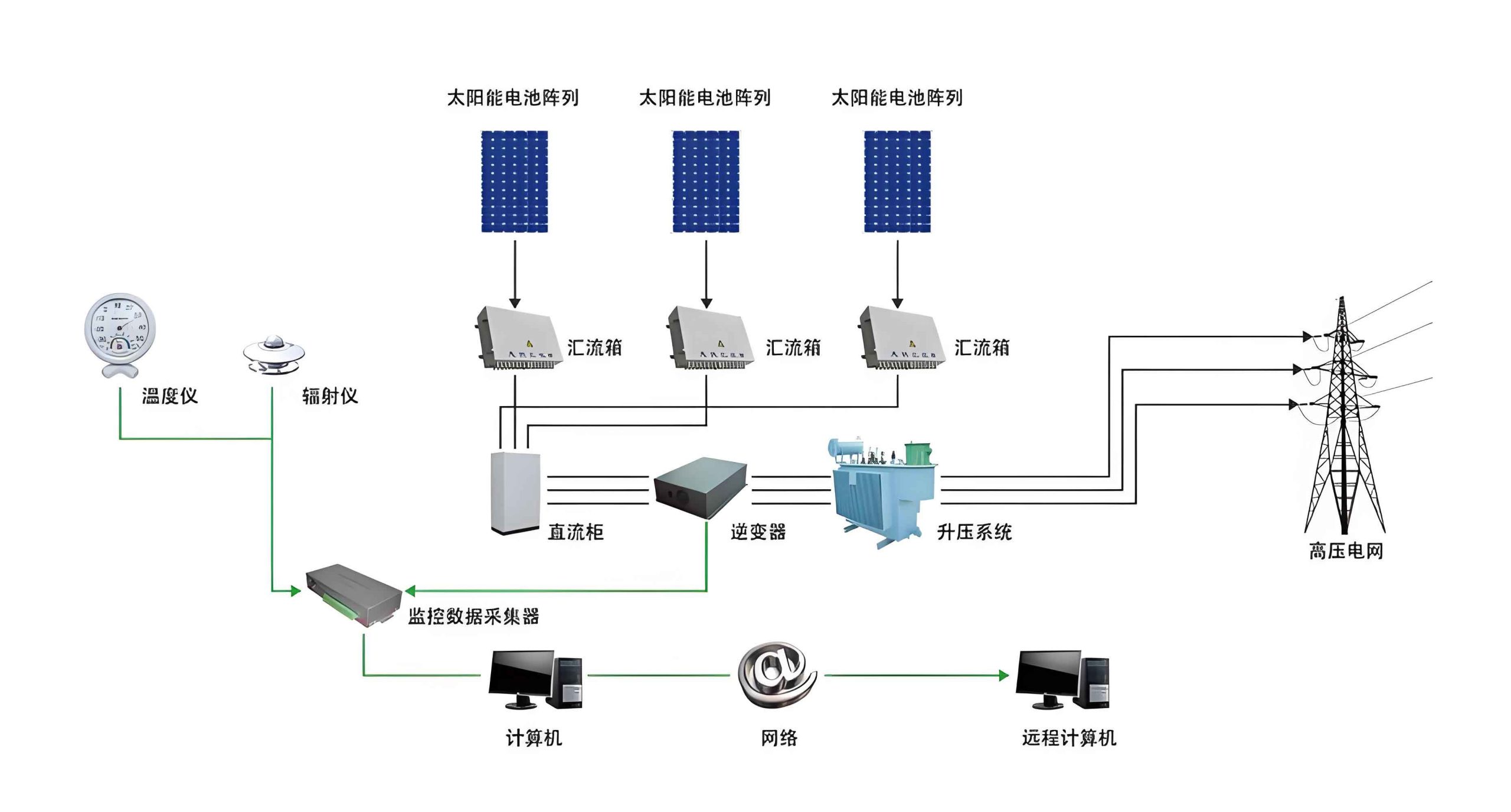
Four adjustable nozzles were allocated per module to ensure complete and even coverage. Prior to testing, the flow rate from each nozzle was calibrated using a measuring cylinder and scale to guarantee a uniform water film across all modules. The total system flow rate was the primary controlled variable. A fixed-tilt PV system, consisting of seven identical modules at the same inclination, served as the non-cooled reference (Track Type Photovoltaic, TPV system, albeit fixed for this comparison). Both systems were instrumented to record module front and back surface temperatures (via thermocouples), output power (via I-V curve tracers), solar irradiance, ambient temperature, and water temperature.
Results and Analysis: Performance of the Cooled Solar System
1. Optimal Cooling Flow Rate
The cooling effectiveness is a balance between enhanced heat removal (beneficial) and increased optical reflection/losses from a thicker water layer (detrimental). Experiments were conducted at varying total flow rates: 0.7, 0.9, 1.1, 1.5, and 1.8 m³/h.
| Flow Rate (m³/h) | Avg. Back Temp. – Cooled System (°C) | Avg. Back Temp. – Reference System (°C) | Avg. Efficiency – Cooled System (%) | Avg. Efficiency – Reference System (%) | Efficiency Gain (Percentage Points) |
|---|---|---|---|---|---|
| 0.7 | 14.7 | 17.9 | 13.5 | 12.6 | +0.9 |
| 0.9 | 13.8 | 17.9 | 14.4 | 12.6 | +1.8 |
| 1.1 | 14.4 | 17.9 | 14.4 | 12.6 | +1.8 |
| 1.5 | 14.4 | 17.1 | 12.9 | 12.9 | 0.0 |
| 1.8 | 13.6 | 17.1 | 13.6 | 12.9 | +0.7 |
The data reveals a clear optimum. At 0.9 m³/h, the cooled solar system achieved the highest average efficiency (14.4%) and the maximum efficiency gain over the reference system (+1.8 percentage points). This corresponds to an estimated water film thickness of approximately 1.1 mm, providing optimal trade-off between cooling and light transmission. Lower flow rates resulted in incomplete surface wetting and higher temperatures, while higher rates created a thick film that excessively blocked sunlight, negating the cooling benefit. This proves that the performance of a water-cooled solar system is not solely a function of temperature reduction but is critically dependent on the hydro-optical properties of the cooling film.
2. Influence of Cooling Water Temperature
The temperature of the cooling water itself is a key parameter. Tests were performed on days with similar irradiance and ambient conditions, but with different average reservoir temperatures.
| Reservoir Temp. | Avg. Module Temp. Reduction (°C) | Avg. Efficiency Gain (Percentage Points) | Peak Power Increase |
|---|---|---|---|
| 22°C | ~5.2 | ~1.8 – 2.1 | Significant |
| 27°C | ~3.5 | ~1.2 – 1.5 | Moderate |
As expected, cooler inlet water provides a greater temperature differential for heat exchange, leading to lower module operating temperatures and consequently higher electrical conversion efficiencies. This highlights the advantage of integrating the cooling system with a low-temperature heat sink or pre-cooling the water for maximum solar system yield during peak insolation periods.
3. All-Day Performance and Temperature Dynamics
A full-day experiment illustrated the dynamic response of the solar system. Before cooling activation, both the test and reference modules showed nearly identical temperature and efficiency profiles. Upon initiating water flow at 0.9 m³/h, the front surface temperature of the cooled module dropped dramatically by approximately 18°C within 15 minutes, demonstrating the immediacy of the cooling effect. The back-surface temperature, which is more representative of the cell operating temperature due to its stability and insulation from direct spray effects, also decreased steadily and remained consistently 3-6°C below the reference module throughout the cooling period. This validates the use of back-surface temperature as a reliable proxy for the cell’s operating temperature in the thermal model for this solar system configuration.
Model Validation and Comparative Summary
Theoretical vs. Experimental Temperature and Efficiency
The theoretical model was solved numerically and compared against measured data. The predicted module temperature profile closely followed the experimental trend, confirming the robustness of the heat transfer model for this solar system. The calculated electrical efficiency from the model also matched the general trajectory of the measured efficiency, though absolute values differed. This discrepancy underscores the model’s simplification regarding the optical losses from the water film; the actual efficiency is governed by the coupled opto-thermal relationship \(\eta_e = f(T, \tau_{water}(d))\), where the water transmittance \(\tau_{water}\) is itself a function of film thickness \(d\).
Comprehensive Benefits of the Water-Cooled Solar System
The comparative study between the front-surface water-cooled PV system and the standard fixed-tilt system reveals multifaceted advantages:
| Aspect | Water-Cooled Solar System | Standard Fixed-Tilt System |
|---|---|---|
| Electrical Efficiency | Increased by 1.2-1.8 percentage points under optimal flow. | Baseline, suffers from temperature-induced losses. |
| Module Temperature | Substantially lower (3-8°C reduction in back temperature). | Operates at higher temperatures, reducing lifespan. |
| Cleaning Effect | Continuous self-cleaning, maintains high light transmittance. | Susceptible to dust accumulation, requiring periodic manual cleaning. |
| Energy Yield | Higher annual energy generation per module. | Lower specific yield. |
Conclusion
The integration of front-surface water cooling presents a highly effective method for performance enhancement in a solar photovoltaic system. This research demonstrates that an optimally designed cooling system, characterized by a specific flow rate that creates a thin, uniform water film (approximately 1 mm), can significantly lower PV module operating temperatures. This thermal management directly translates into a measurable increase in electrical conversion efficiency, with gains of over 1.8 percentage points observed under test conditions. Furthermore, the system inherently provides a cleaning action, mitigating another common cause of performance loss. The developed theoretical model aligns well with experimental data, providing a valuable tool for designing such systems for different climates and scales. While water consumption and system cost are factors for consideration, the combined benefits of increased energy yield, potential module lifespan extension due to lower thermal stress, and reduced maintenance through automated cleaning make front-surface water cooling a compelling strategy for optimizing the performance and economics of solar power plants, particularly in hot and dusty environments. The implementation of this technology can lead to a more efficient and robust solar system, contributing to improved capacity factors and a lower levelized cost of electricity from photovoltaic installations.