
The proliferation of renewable energy sources has made the power electronic inverter, serving as the primary grid interface, indispensable in modern power systems. Among various control strategies for on-grid inverters, droop control has gained significant prominence. It emulates the frequency and voltage regulation characteristics of synchronous generators, enabling the inverter to provide essential grid support. However, the transient stability of droop-controlled on-grid inverters during severe grid disturbances, such as symmetrical faults, presents a critical challenge. Two primary issues emerge: transient power angle instability and fault overcurrent. Existing solutions often address these problems in isolation, neglecting their inherent coupling. This article proposes a comprehensive transient control strategy that simultaneously ensures transient power angle stability and provides effective fault current limitation for droop-controlled on-grid inverters.
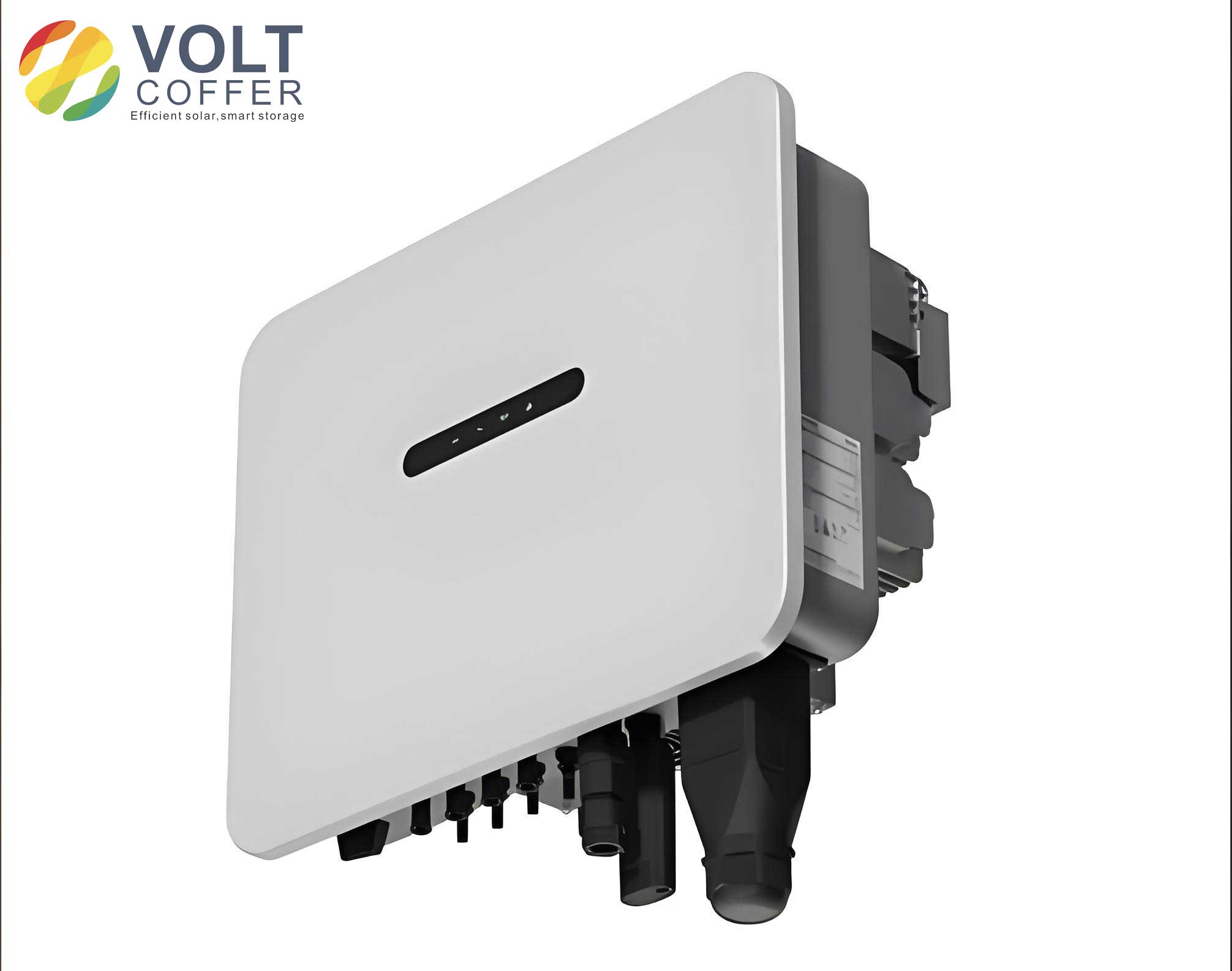
Transient Characteristics Analysis of Droop-Controlled On-Grid Inverters
The fundamental principle of droop control for an on-grid inverter involves two outer loops: the active power-frequency (P-ω) loop and the reactive power-voltage (Q-V) loop. The standard control equations are:
$$ \omega = \omega_0 + K_{pf}(P_0 – P) $$
$$ V = V_0 + K_{qv}(Q_0 – Q) $$
where ω and V are the output angular frequency and voltage magnitude of the on-grid inverter, respectively. ω₀ and V₀ are their nominal setpoints. P and Q are the measured output active and reactive power, while P₀ and Q₀ are their reference values. Kpf and Kqv are the droop coefficients. The power delivered to the grid through an equivalent line reactance Xg is:
$$ P = \frac{3}{2} \cdot \frac{E V}{X_g} \sin \delta $$
$$ Q = \frac{3}{2} \cdot \frac{V^2 – E V \cos \delta}{X_g} $$
Here, E is the grid voltage magnitude, and δ is the power angle between the inverter output voltage and the grid voltage.
Mechanism of Transient Power Angle Instability
During a grid fault, the voltage E drops significantly. This causes a sudden reduction in the output active power P of the on-grid inverter. According to the P-ω droop law, the imbalance between P₀ and P leads to an increase in frequency, which integrates into a growing power angle δ. The stability criterion hinges on the existence of a stable equilibrium point where the derivative of the power angle, \(\dot{\delta}\), becomes zero. The dynamic equation, initially neglecting the Q-V loop (assuming V constant at V₀), is:
$$ \dot{\delta} = K_{pf}(P_0 – P) = K_{pf} \left( P_0 – \frac{3}{2} \cdot \frac{E V_0}{X_g} \sin \delta \right) $$
If, post-fault, the maximum transmissible power \(P_{max} = \frac{3}{2} \cdot \frac{E V_0}{X_g}\) is less than P₀, then \(\dot{\delta}\) remains always positive. Consequently, the power angle δ increases monotonically, leading to transient instability. The unbalanced power \(P_0 – P\) is the root cause.
Impact of the Reactive Power Control Loop
In reality, the Q-V control loop significantly influences transient stability. During a fault, the reactive power Q changes, which modulates the output voltage V according to the Q-V droop equation. A varying V further affects the active power P, creating a coupling that can deteriorate stability. By combining the Q-V droop and reactive power equations, we derive the relationship between V and δ:
$$ V = \frac{K_{qv} E \cos \delta + \sqrt{(K_{qv} E \cos \delta)^2 + 4 K_{qv} [X_g V_0 + K_{qv} X_g (Q_0 – \frac{3V_0^2}{2X_g})] } }{2} $$
Analysis shows that \(\frac{dV}{d\delta} < 0\) for δ ∈ [0, π]. As the power angle δ increases during a transient, the output voltage V decreases. This reduction in V further decreases the active power P, increasing the unbalanced power and accelerating the growth of δ. Therefore, the reactive power control loop in a standard droop-controlled on-grid inverter often exacerbates transient instability.
Fault Current Characteristics
During a symmetrical fault, the fault current IF of the on-grid inverter can be derived from the equivalent circuit:
$$ I_F = \frac{\sqrt{V_F^2 + E’^2 – 2 V_F E’ \cos \delta’}}{X_g} $$
where VF and E’ are the inverter output voltage and grid voltage during the fault, and δ’ is the transient power angle. This equation reveals the coupling between fault current, power angle, and output voltage. For a given fault depth (E’), the fault current magnitude increases with the power angle δ’. Conversely, if the power angle is controlled to remain constant, the fault current is inversely related to the output voltage VF. This relationship is key to designing a coordinated control strategy.
Proposed Comprehensive Transient Control Strategy
The objective is to ensure that the on-grid inverter maintains transient power angle stability while limiting the fault current to a safe threshold Ilimit (e.g., 1.3 per unit of rated current). The strategy involves two coordinated modifications to the standard droop control.
1. Transient Power Angle Dynamic Compensation
To prevent the monotonic increase of the power angle, we introduce a dynamic compensation term into the active power reference of the droop control. The goal is to compensate for the unbalanced power dynamically, forcing the power angle to settle near its pre-fault steady-state value δa. The modified P-ω control law becomes:
$$ \omega = \omega_0 + K_{pf}[(P_0 + P_\delta) – P] $$
The compensation power Pδ is designed to be proportional to the power angle deviation Δδ = δ’ – δa:
$$ P_\delta = K_\delta \cdot \Delta \delta $$
where the compensation coefficient Kδ is derived based on the linearized power-angle relationship during the fault, considering the coupled effect from the voltage:
$$ K_\delta = \frac{3}{2} \cdot \frac{E’ V_F}{X_g} \cos \delta_a $$
This term effectively reduces the net unbalanced power seen by the integrator, stabilizing the power angle. The stability of this augmented control system can be proven using a Lyapunov energy function. Defining state variables x₁ = δ – δa and x₂ = Δω, and considering a low-pass filter in the power measurement with time constant T, the system dynamics are:
$$ \begin{aligned}
\dot{x}_1 &= x_2 \\
T \dot{x}_2 &= -x_2 – K_{pf} \left( \frac{3E’V_F}{2X_g}(\sin \delta – \sin \delta_a) – K_\delta x_1 \right)
\end{aligned} $$
Constructing the Lyapunov function candidate:
$$ V(x_1, x_2) = \frac{1}{2} x_2^2 + \frac{K_{pf}}{T} \int_0^{x_1} \left[ \frac{3E’V_F}{2X_g}(\sin(\delta_a+\tau) – \sin \delta_a) – K_\delta \tau \right] d\tau $$
Its derivative is:
$$ \dot{V} = -\frac{1}{T} x_2^2 \leq 0 $$
By LaSalle’s invariance principle, the system is asymptotically stable, proving that the proposed compensation enhances the transient stability of the on-grid inverter.
2. Adaptive Voltage Reference Adjustment for Fault Current Limiting
With the power angle stabilized near δa by the first control action, the fault current equation simplifies. To enforce IF ≤ Ilimit, we can adaptively adjust the voltage reference in the Q-V control loop. From the fault current equation with δ’ ≈ δa:
$$ I_F = \frac{\sqrt{V_F^2 + E’^2 – 2 V_F E’ \cos \delta_a}}{X_g} $$
Setting IF = Ilimit and solving for the required output voltage VF* yields:
$$ V_F^* = \frac{nk + \sqrt{n^2 k^2 – 4(k^2 E^2 – 1.69 X_g^2 I_{gN}^2)}}{2} $$
where \( n = \frac{V_0^2 + E^2 – X_g^2 I_{gN}^2}{2 V_0 E \cos \delta_a} \), k = E’/E is the voltage dip ratio, and IgN is the rated current. The adaptive voltage reference V’ for the Q-V loop during the fault is then set as:
$$ V’ = \begin{cases}
V_F^*, & \text{if } V_F^* > V^* \\
V^*, & \text{otherwise}
\end{cases} $$
Here, V* is the nominal voltage reference from the steady-state droop equation. This adaptive adjustment ensures that during severe faults, the on-grid inverter reduces its output voltage to limit the current, while during mild faults, it continues to operate with normal voltage support.
3. Integrated Control Strategy and Comparison
The complete control strategy for the on-grid inverter is summarized in the following block diagram and logic flow. The system continuously monitors the grid voltage. Upon detecting a fault (e.g., voltage below 0.9 p.u.), the transient control mode is activated: the power angle dynamic compensator is engaged in the P-ω loop, and the adaptive voltage reference VF* is calculated and applied to the Q-V loop if it is lower than the nominal reference. This integrated approach addresses both stability and fault current concerns concurrently. The following table compares the proposed method with other existing transient control methods for on-grid inverters.
| Control Method | Transient Power Angle Stability | Fault Current Limiting Capability | Considers Q-V Loop Impact |
|---|---|---|---|
| Conventional Droop | Unstable for severe faults | Weak | No |
| Adaptive Droop Coefficient [Ref.] | Stable | Weak for deep faults | Yes |
| Virtual Impedance Current Limiting [Ref.] | May become unstable | Strong | No |
| Current Reference Limiting [Ref.] | Unstable | Strong | No |
| Proposed Integrated Strategy | Stable | Strong | Yes |
Simulation Verification
The proposed strategy is validated through simulations of a droop-controlled on-grid inverter system in MATLAB/Simulink. The key parameters are: Srated = 10 kVA, V0 = 220 V, E = 220 V, f0 = 50 Hz, Xg = 8 mH, Kpf = 2000 (N·m·s)/rad, Kqv = 4500 var/V, Ilimit = 1.3 p.u. A symmetrical three-phase fault is applied at t = 1 s and cleared at t = 3 s.
Case 1: Moderate Fault (Grid Voltage Drops to 0.4 p.u.)
The performance under a 0.4 p.u. voltage dip is evaluated for three control schemes: conventional droop, adaptive droop control from literature, and the proposed integrated control. The results are summarized below.
| Control Method | Final Power Angle (p.u.) | Max. Fault Current (p.u.) | Stable? | Current within Limit? |
|---|---|---|---|---|
| Conventional Droop | 2.15 | 2.02 | Yes | No |
| Adaptive Droop [Ref.] | 0.78 | 1.28 | Yes | Yes |
| Proposed Control | ~1.00 | 1.30 | Yes | Yes |
The proposed control successfully maintains the power angle close to its pre-fault value (1.0 p.u.) and strictly limits the fault current to the 1.3 p.u. threshold. The adaptive droop method also limits current but does not preserve the original power angle. The conventional on-grid inverter, while stable in this moderate case, allows excessive overcurrent.
Case 2: Severe Fault (Grid Voltage Drops to 0.2 p.u.)
This case tests the robustness under a deep fault. The comparative results are shown below.
| Control Method | Power Angle Behavior | Max. Fault Current (p.u.) | Stable? | Current within Limit? |
|---|---|---|---|---|
| Conventional Droop | Oscillatory Divergence | >2.5 | No | No |
| Adaptive Droop [Ref.] | Stable at ~0.75 p.u. | 1.76 | Yes | No |
| Proposed Control | Stable at ~1.00 p.u. | 1.30 | Yes | Yes |
Under this severe disturbance, the conventional on-grid inverter loses transient stability. The adaptive droop method stabilizes the power angle but fails to limit the fault current within the safe threshold, which could damage the inverter switches. In contrast, the proposed integrated control strategy for the on-grid inverter demonstrates superior performance: it maintains transient power angle stability while effectively constraining the fault current to the predefined safe limit. Furthermore, by controlling a higher output voltage than the pure current-limiting methods would allow, the proposed strategy enables the on-grid inverter to inject more reactive power during the fault, which actively supports grid voltage recovery.
Conclusion
This article has analyzed the coupled challenges of transient power angle instability and fault overcurrent in droop-controlled on-grid inverters during grid faults. The reactive power-voltage control loop was shown to negatively impact transient stability. A novel integrated transient control strategy was proposed, featuring a dynamic power angle compensator in the active power loop and an adaptive voltage reference adjuster in the reactive power loop. The compensator ensures transient power angle stability by counteracting unbalanced power, a principle rigorously supported by Lyapunov stability analysis. The voltage adjuster guarantees that the fault current remains within a safe operational limit. Comprehensive simulation studies confirm that the proposed strategy enables the on-grid inverter to maintain stable operation and provide controlled fault current under both moderate and severe voltage sags, outperforming methods that address only one aspect of the transient problem. This work enhances the fault ride-through capability and reliability of on-grid inverters in modern power systems with high penetration of renewable energy.