
For the operation of energy storage systems, SOC is an important indicator for evaluating the health status of energy storage. The commonly used constant parameter power difference control strategy determines the action value of the energy storage system by partitioning the load, but this strategy does not consider the SOC state of the energy storage system. This chapter uses an improved variable parameter power difference control strategy to partition the SOC based on the load partitioning, in order to avoid exceeding the limit of the energy storage system.
1.Load zoning and SOC state interval division
1.1 Load zoning
Based on the fast charging and discharging characteristics of energy storage equipment, the energy storage system can charge and store energy during low load periods, alleviating the pressure of new energy consumption; Discharge energy during peak load hours to reduce the pressure on the power grid caused by the load. Thus, peak shaving and valley filling can be achieved for the power grid, ensuring its operational reliability. Among them, the participation of energy storage in peak shaving and valley filling is divided into two stages, namely daily control strategy and real-time optimization. The first stage mainly determines the output time period and output size of the energy storage system through the peak valley values of the load curve; In the second stage, based on the determined charging and discharging period and output size in the first stage, the actual output of the energy storage system is determined by considering the battery status.
Figure 1 shows the load partitioning method under the constant parameter power difference control strategy, which mainly considers the capacity and power constraints of the energy storage system. The load partitioning process is as follows:
(1) Calculate the daily average load Pavg by accumulating the values of each point through the daily load prediction curve, and determine the iteration step size at the same time Δ P. And the peak and valley power of the load.
(2) By iterating step by step, the next step of calculation is carried out when the charging and discharging levels are less than the battery capacity.
(3) If the maximum charging capacity is ≥ the maximum discharge capacity, and the difference is close to 0, then the upper charging limit power P1 and the lower discharging limit power P2 can be determined.
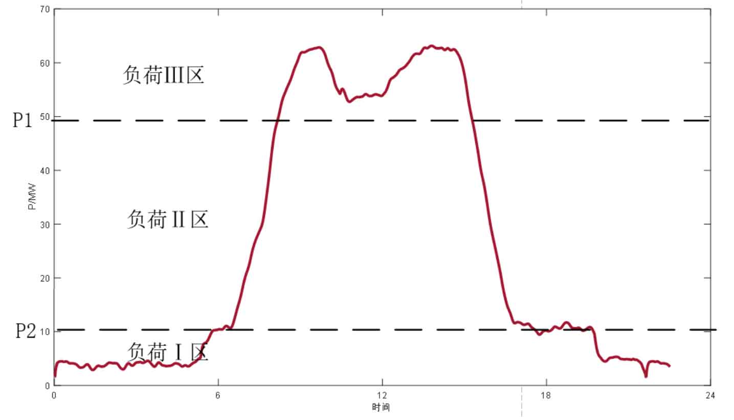
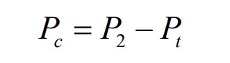
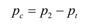
(1) Load Zone I (energy storage charging range): At this time, P2 ≤ Pt is met, where Pt is the load power at time t. At this time, the energy storage system charges to fill the load valley, and the charging power is:
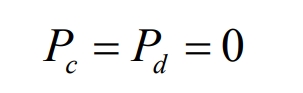
(2) Load Zone II (energy storage non action interval): This interval P2<Pt<P1, at which time the energy storage system does not act as:
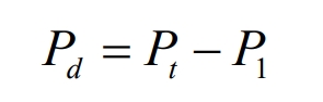
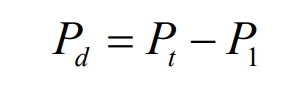
(3) Load Zone III (Energy Storage and Discharge Zone): In this zone, Pt ≥ P1 is met, and the battery energy storage system discharges to flatten the load peak. The discharge power is:
The constant parameter power difference control strategy predicts the load value by calculating the average output, thereby determining the output of the energy storage system. However, this method does not take into account the SOC state of the system. When the energy storage system is at peak load or valuation stage for a long time, the SOC exceeds the limit, which has an adverse impact on the system’s lifespan.
On the basis of the constant parameter power difference control strategy, this article uses an improved variable parameter power difference control strategy, considering the SOC state, to reduce the duration of the energy storage system appearing in the high or low SOC range, thereby extending the service life of the energy storage system.
1.2 SOC state interval division
By introducing two variables, Sup and Down, the SOC state interval is divided into five intervals, as shown in the following figure:
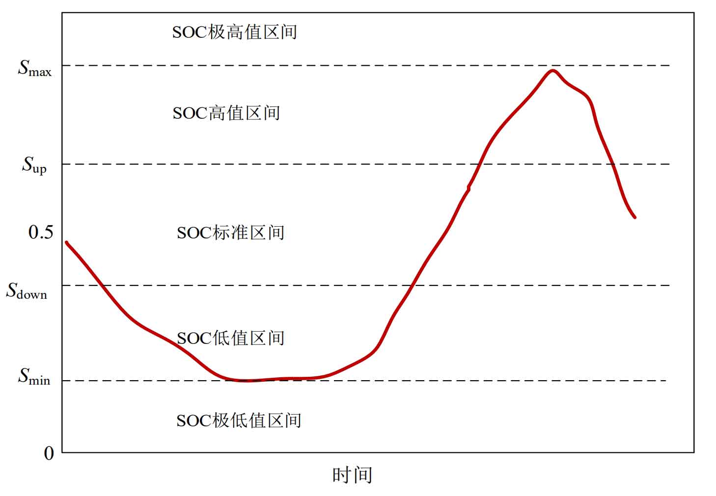
As shown in Figure 2, the SOC state interval is divided as follows:
(1) When the SOC value at time t is within Smax ≤ S (t)<1, this range is the extremely high SOC value range;
(2) When the SOC value at time t is within Sup ≤ S (t)<Smax, this interval is the high value range of SOC;
(3) When the SOC value at time t is within Sdown ≤ S (t)<Sup, this interval is the SOC standard interval;
(4) When the SOC value at time t is within Smin ≤ S (t)<Sdown, this interval is the low value range of SOC;
(5) When the SOC value at time t is 0 ≤ S (t)<Smin, this range is the extremely low SOC value range.
The SOC state interval is divided into five intervals: SOC extremely high value region, SOC high value region, SOC standard region, SOC low value region, and SOC extremely low value region. Their relationship satisfies the following constraints:
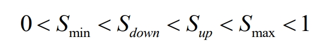
Among them, Smax and Smin are the maximum and minimum allowable SOC values for the energy storage system; Sup and Down are parameters that divide the SOC state interval.
The principle of variable parameter power difference control strategy is to adjust the charging and discharging power in the high and low value regions of SOC, and minimize the time when SOC is in the extremely high and low regions as much as possible. To this end, control parameters a, b, c, and d are introduced, and their control principles are as follows:
(1) SOC extremely high value zone: The system does not perform charging operations within this range.
In load zone I, the energy storage system does not operate, and the main grid and photovoltaic array provide power to the energy storage power station.
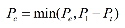
In load zones II and III, the energy storage system discharges. According to the power constraints of the energy storage system, its discharge power is:
Pd=min (Pe, Pt-P2), where Pe is the rated power of the energy storage system; Pt is the load power.
(2) SOC high limit zone: Within this zone, the system performs different charging and discharging operations based on the different load zones it is in.
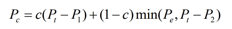
In load zone I, the energy storage system charges, but excessive charging power can cause SOC to enter the upper limit zone. The charging power in this zone is:
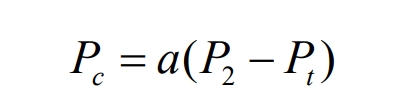
Among them,0<a<1, thus taking into account the SOC state while filling the valley in load zone I.
In load zone II, the system does not operate.
In load zone III, the system increases power discharge to avoid entering the extremely high value zone as much as possible. Based on the power and load range constraints during discharge, the discharge power at this time is:
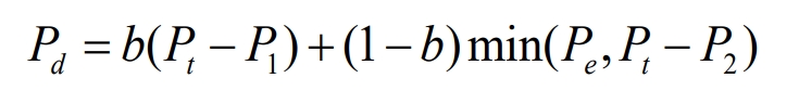
Among them, 0<b<1, Pt P1<Pe, the discharge power range in this range [Pt-P1, min (Pe, Pt-P2)]
(3) SOC standard zone: Within this zone, the system performs different charging and discharging operations based on the different load zones it is in.
In load zone I, the energy storage system is charged with a charging power of:
In load zone II, the energy storage system does not operate.
In load zone III, the discharge power of the energy storage system is:
(4) SOC low value zone: In this zone, the system performs different charging and discharging operations based on the different load zones it is in, and its energy storage action is opposite to the SOC high limit zone.
In Load Zone I, the energy storage system performs charging operations with a charging power of:
Where 0<c<1.
In load zone II, the energy storage system does not operate.
In Load Zone III, the energy storage system performs a discharge operation with a discharge power of:
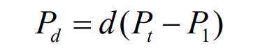
Among them, 0<d<1.
(5) SOC extremely low value zone: In this zone, the energy storage system does not perform discharge operation, which is opposite to the SOC extremely high value zone. In load zone I and zone II, the charging power of the energy storage system is:
In load zone III, the energy storage system does not operate.
As mentioned above, the two parameter variables Sup and Sdown divide the state of charge of the energy storage system, and further control the charging and discharging power of each interval through the four control parameters a, b, c, and d. This achieves the goal of considering both the load interval and the SOC state. Through rolling updates of the six parameters Sup, Sdown, a, b, c, and d, an effective strategy of considering the SOC state is finally achieved.
2. Parameter optimization of variable parameter control strategy
In order to make the control strategy of this article forward-looking, ultra-short term predicted power is introduced to calculate the output of photovoltaic power plants in the next 4 hours, updated every 15 minutes. Considering the fluctuation of load, combined with the daily load prediction curve, these 6 variables are optimized every 15 minutes based on the objective function.
2.1 Objective function
Evaluate the peak shaving and valley filling effects and changes in SOC state under the variable parameter control strategy, while considering the relevant characteristics of photovoltaic power generation, establish the following sub objective functions.
(1) Peak shaving and valley filling evaluation indicators
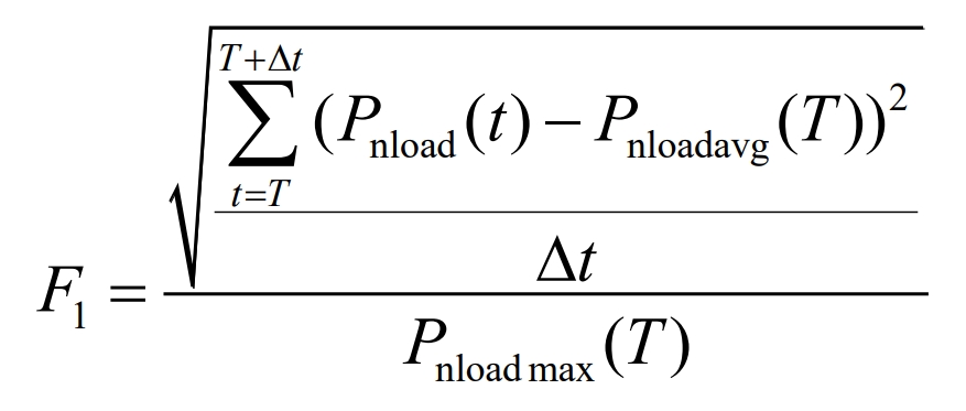
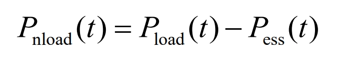
In the formula, Pnload (t) is the load side power at time t; Pnloadavg (T) is [T, T+ Δ T] The average power of the load during the time period; Pnload max (T) is the maximum load power value during this period; Δ T is the length of each period of time.
In this equation, the load power is the total power (including energy storage power and load power), which is:
(2) SOC evaluation indicators
Define the SOC fluctuation evaluation index F2 as:
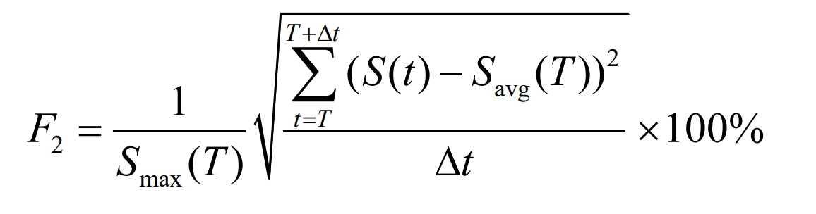
Among them, Savg (T) is [T, T+ Δ T] The average SOC value during the time period; Smax (T) is the maximum SOC value during that time period.
(3) Power supply dissatisfaction
Considering the randomness and uncertainty of photovoltaic system output on the impact of this control strategy, in order to improve the utilization rate of new energy, the objective function F is introduced:
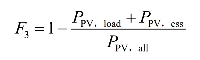
In the formula, F3 is the ratio of the absorbed power of the photovoltaic system at any given moment to the total output power of the photovoltaic system at that moment. Among them, PPV load and PPV ess refer to the photovoltaic power absorbed by the load and battery.
PPV all is the total output power of the photovoltaic system at that time.
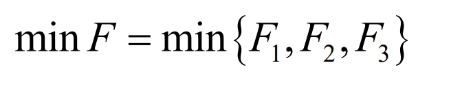
In summary, the objective function of this strategy is composed of a combination of F1, F2, and F3, namely:
For the different characteristics of the objective function represented by F1, F2, and F3, select the weight coefficient ω I (i=1, 2, 3), i.e.:
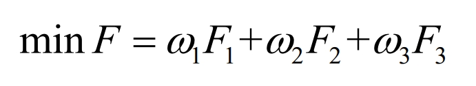
Among them, ω 1+ ω 2+ ω 3=1, in order to determine each objective subfunction, this article adopts the subjective and objective comprehensive weighting method, namely:
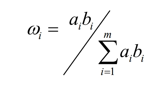
In the formula, ai is the weight obtained by the subjective weighting method; Bi is the weight obtained by the objective weighting method.
2.2 Constraints
The control strategy proposed in this article mainly considers grid constraints, self constraints of large-scale energy storage systems, and constraints on six control parameters.
(1) Power balance constraints of the power grid
To ensure the normal operation of large-scale energy storage system equipment, it is necessary to meet the power balance of the power grid, namely:
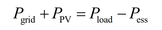
Among them, Pgrid is the output power of the main network to the energy storage system; PPV is the output power of the photovoltaic array system; Pload is the load power; Pess is the output of the energy storage system.
(2) Constraints of the energy storage system itself
The self constraints of the energy storage system are as follows:
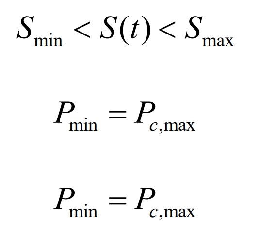
Among them, Smin is generally taken as 20% to 30%, and Smax is generally taken as 75% to 80%; Pc, max Pd, max are the maximum allowable charging and discharging power values of the energy storage system.
The relationship between SOC, capacity, and charging and discharging power of the energy storage system is as follows:
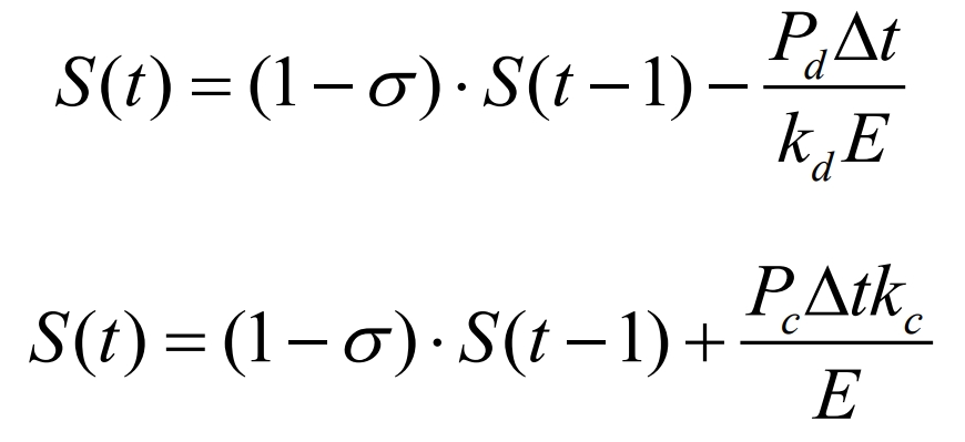
among σ Is the self discharge rate of the energy storage system; S (t) is the SOC value at time t; E is the total capacity of the energy storage system; Kc and kd are the charging and discharging efficiency of the energy storage system, respectively.
(3) Photovoltaic power constraints
Due to the randomness of photovoltaic power generation systems, if the reverse power of photovoltaic arrays to the power grid is too large, it will pose a threat to the reliability of power grid operation. Therefore, the photovoltaic reverse power is limited as follows.

Among them, PPV grid refers to the reverse power transmitted by the photovoltaic system to the power grid at a certain time; PPV grid_ Max is the maximum allowable reverse power of the photovoltaic system for the regional power grid.
2.3 Dynamic adaptive particle swarm optimization algorithm
Based on the above objective functions and constraints, this paper adopts dynamic adaptive particle swarm optimization algorithm to perform rolling optimization on the six parameters introduced, namely Sup, Down, a, b, c, and d.
Particle Swarm Optimization (PSO) is an optimization algorithm that randomly searches and quickly optimizes, with characteristics such as fast convergence speed, simplicity, and ease of implementation. However, due to the fast convergence algorithm, it is difficult to find the global optimal solution in particle swarm optimization due to the dispersed optimization of each particle. If the inertia weight in particle swarm optimization algorithm is large, it will be beneficial for global search, but it will lead to a decrease in the convergence speed of the algorithm; If the inertia weight is small, it will accelerate convergence but make the algorithm less global.
The adaptive particle swarm optimization algorithm searches for the optimal solution through the assistance of particles, and continuously updates the speed and position of the examples during the optimization iteration process. Update the formula to:
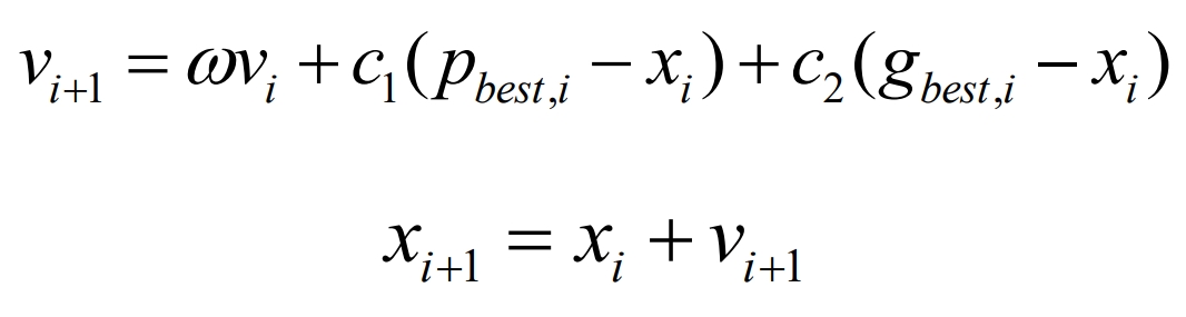
Among them, vi is the current velocity of the particle; Xi is the current position of the particle; Pbest i is the optimal solution for the current individual; Gbest i is the optimal solution for the current population; ω Is the inertia weight; C1 and c2 are acceleration factors.
To overcome the shortcomings of fixed inertia weights, the weight coefficients are adaptively updated according to the following formula:
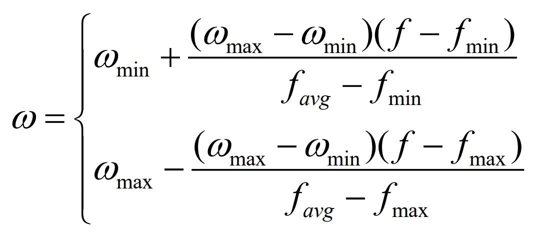
In the formula, f is the current particle fitness; Favg is the average fitness of the current population; Fmin is the minimum fitness value of the current population; ω Min is the minimum value of inertia weight; ω Max is the maximum value of inertia weight.
The specific steps of the algorithm are as follows.
Step 1: Set the total number of particles n, iteration number m, and acceleration factors c1 and c2;
Step 2: Set the upper and lower limits of particle positions in the population, initialize 6 parameters, and obtain the SOC value, photovoltaic output power, and load size at T0 time;
Step 3: Start iteration and optimize the objective function to obtain the corresponding optimal solution;
Step 4: Update the inertia weight based on the updated particle velocity and position, and determine the weight values of the sub objective function;
Step 5: Bring the weights into the total objective function, use the algorithm to optimize, and obtain the optimal solutions for six parameter variables
Step 6: Determine whether the iteration result meets the termination condition. If so, end the iteration and output the result; If not, return to step 5 and iterate again.
3.Example analysis
This article analyzes a photovoltaic power plant with an installed capacity of 200MW in Qinghai, and verifies the effectiveness of the variable parameter power difference control strategy proposed in this paper through simulation. The data used for simulation is the output power and predicted power of the photovoltaic energy storage station on a certain day in May, with a power sampling interval of 60 seconds.
The configuration parameters of the photovoltaic energy storage station are as follows: the installed capacity of the photovoltaic system is 200MW; The energy storage system is a lithium iron phosphate battery with a rated power of 50MW and a rated capacity of 50WMh. Set Sup=0.8; Sdown=0.2; σ= 0 Improved adaptive particle swarm optimization algorithm with n=50 particles and m=300 iterations; The acceleration factor c1=c2=2.
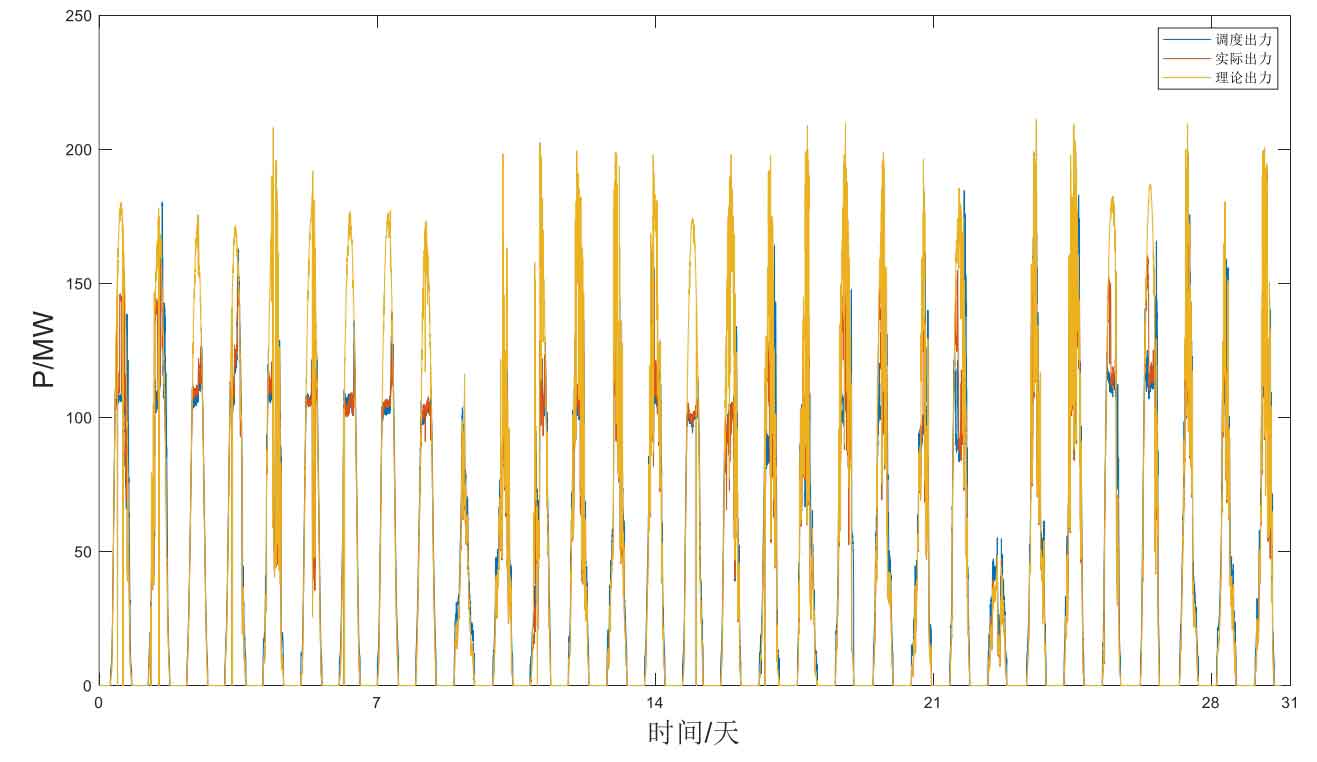
Figure 3 shows the daily photovoltaic output curve of a certain photovoltaic power station in Qinghai for a certain month. It can be seen that in general, the photovoltaic output can reach the rated output power, while on the 13th and 24th, the photovoltaic output significantly decreased. This is due to the environmental impact, with a significant decrease in solar lighting during cloudy and rainy days.
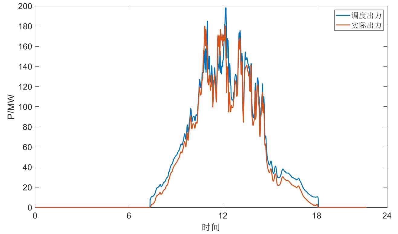
Figure 3 shows the output curve of a photovoltaic power plant under normal weather conditions, with the blue line indicating the dispatch output and the red line indicating the actual output. From the curve trend, it can be seen that 7-18h is the working output period of the photovoltaic power plant, which is also consistent with the daytime solar irradiation period.
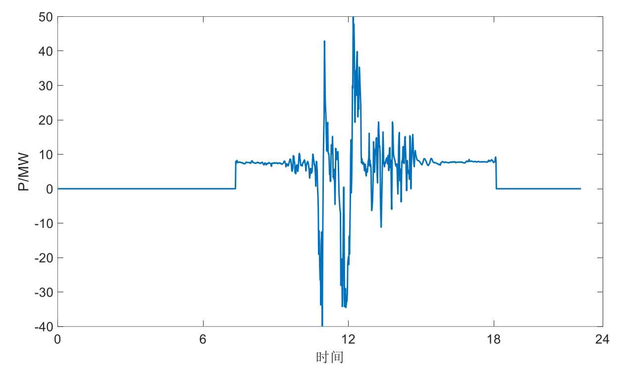
Figure 5 shows the daily charging and discharging output curve of the energy storage power station, which is the difference between the scheduled output and actual output of the photovoltaic power station in Figure 4. Similar to the above figure, during the daytime working period of the photovoltaic system, the output of the energy storage system is in a discharge working state. During the midday period when the load and light intensity are at their peak, the energy storage system completes charging and discharging operation instructions based on the actual situation.
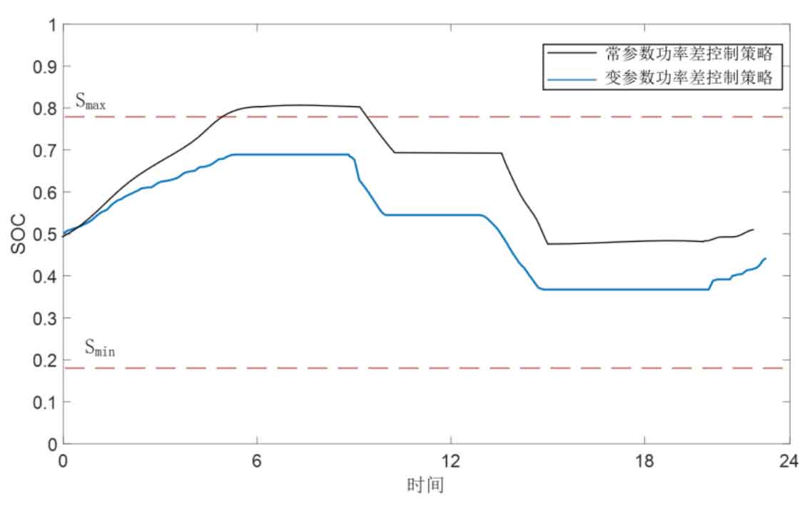
Figure 6 shows that the SOC of the energy storage system under the variable parameter power control strategy remains between the upper and lower boundaries [0.2, 0.8] within a day, achieving effective control of SOC. Compared with the constant parameter power difference control strategy, the curve exceeds the extremely high SOC range, which is detrimental to the energy storage life. The energy storage system performs discharge operations from 9:00 to 12:00 and from 13:00 to 15:00, reducing the load during the peak period of the original load curve. Charging operations are carried out from 22:00 to 6:00, increasing the load during the low period of the original load curve. From the comparison curves, it can be seen that the improved control strategy in this article takes into account both the SOC index and the effect of peak shaving and valley filling.
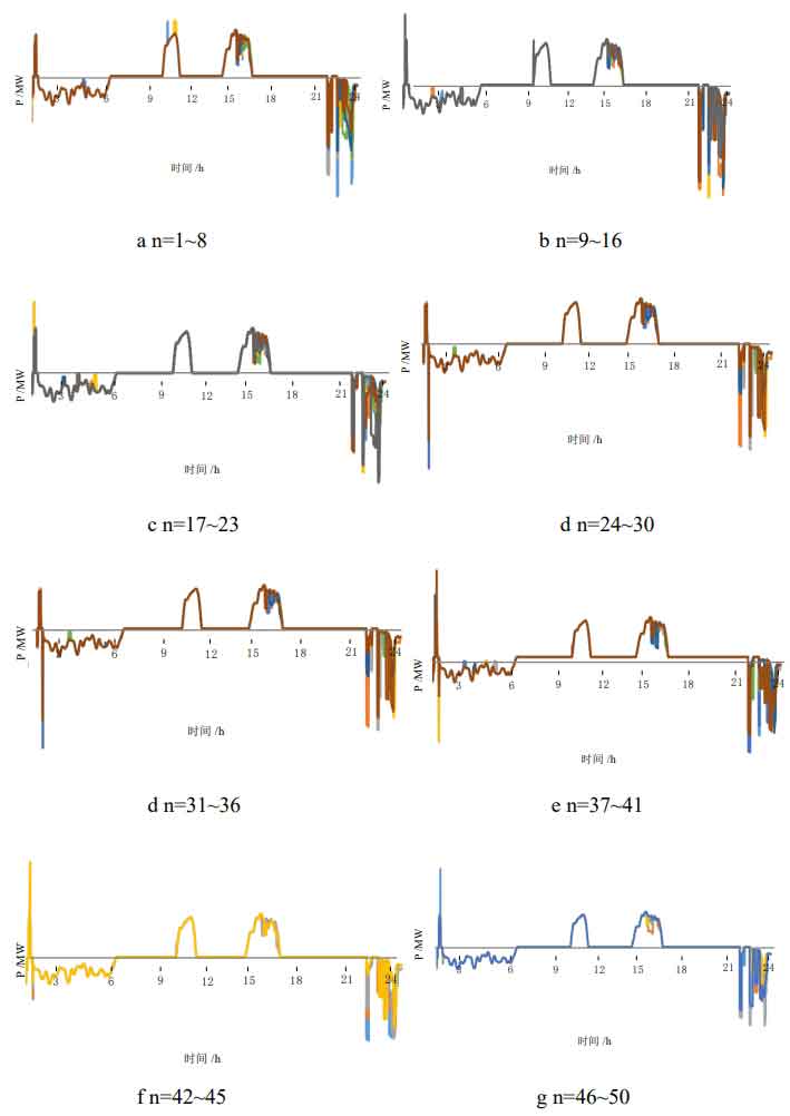
Figure 7 shows the output of each energy storage system under the condition of setting the number of particles n=50 under the program of adaptive particle swarm optimization algorithm. From the overall trend of these 50 cases, it can be seen that the energy storage system recharges during the night time periods of 0-6h and 22-24h to smooth out the low load of the power grid; Discharge during the daytime period of 10-12 hours and 13-17 hours to restore the peak load of the power grid. The effect of peak shaving and valley filling has been achieved.
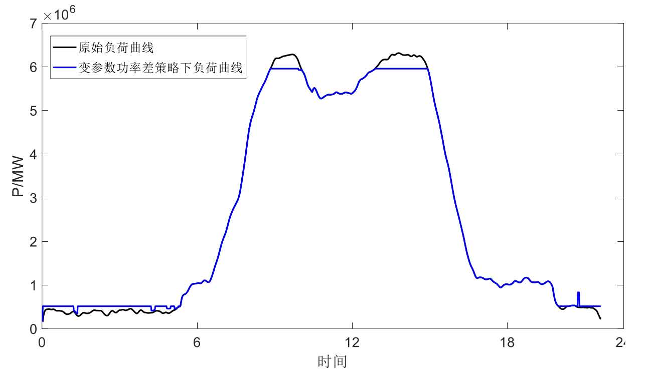
Figure 8 shows the power curve compared to the original load under the variable parameter power difference strategy. It can be seen that during peak hours, the variable parameter control strategy weakens the original load peak and achieves peak shaving effect. At night, it also slightly increases compared to the original load curve, achieving valley filling effect.
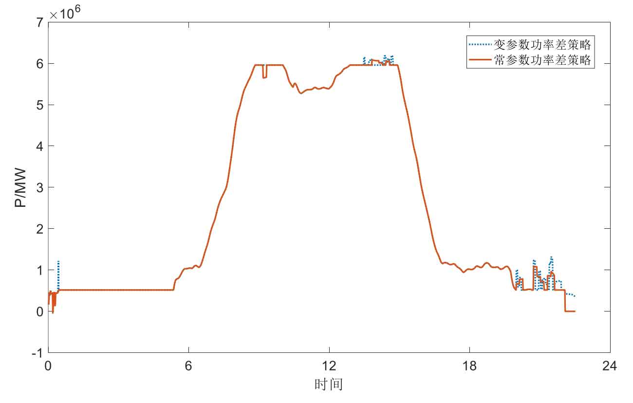
Figure 9 shows the comparison of the optimization effects of the constant parameter power difference and variable parameter power difference strategies. It can be seen that in the overall trend of the curve, the two control strategies are basically the same, both achieving peak shaving and valley filling effects on the load. However, compared to the variable parameter power difference control strategy, the constant parameter strategy has a worse peak shaving and valley filling effect, and the curve fluctuation is more obvious. As for the concave and convex areas appearing in the curve, it is a manifestation of the energy storage system reducing or increasing output when the charging and discharging parameters and the state of charge parameters are activated.
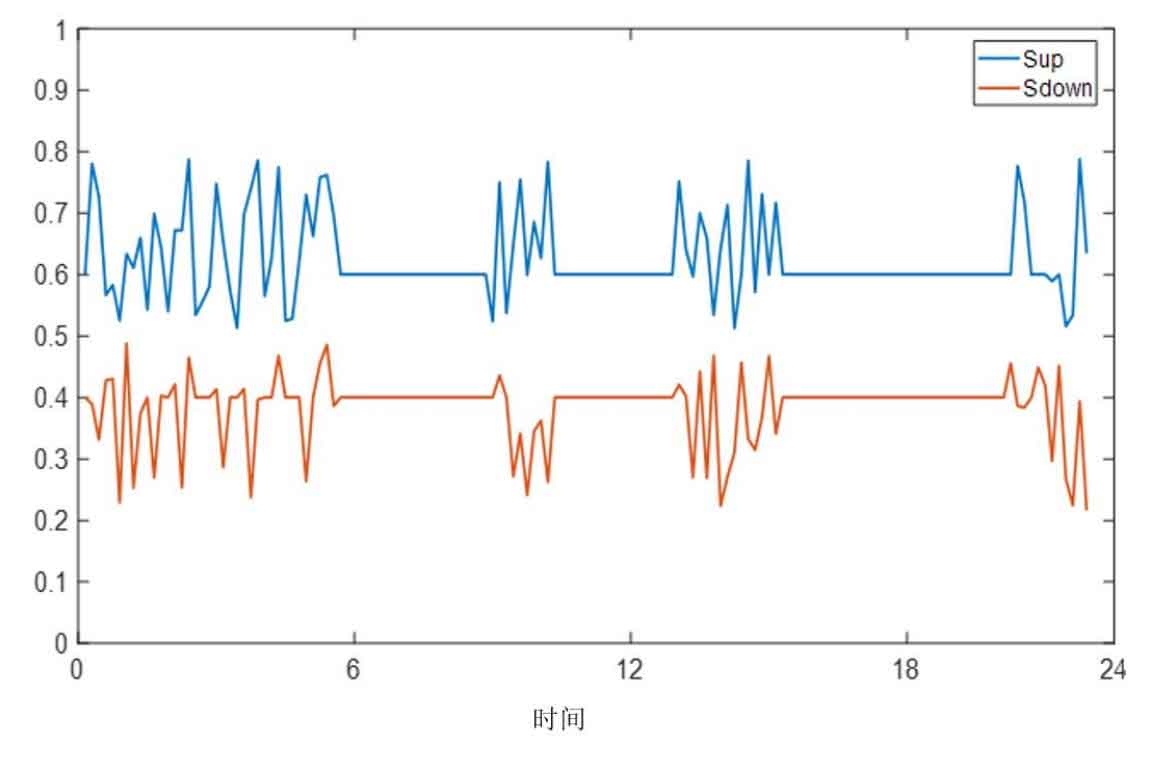
The function of the control variables Sup and Sdown is to divide the charging state interval of the energy storage system. As shown in Figure 9, during certain periods of 9-13h, Sdown is at a lower value level under the influence of the optimization variables. This is equivalent to narrowing the range of the SOC lower limit interval, reducing the probability of the energy storage system entering the SOC lower limit region, and thus making it more effective in entering the SOC normal range.
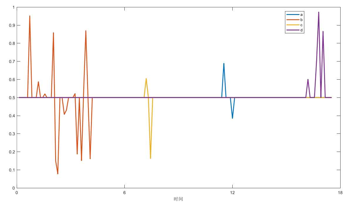
As shown in Figure 10, from 0 to 6 hours, the energy storage system is charged. Starting from around 2 00 hours, the SOC of the energy storage system increases to around 0.6, and the Sup value updates to 0.6. At this point, the energy storage system enters the upper limit range of SOC, and parameter a executes an action to effectively reduce the energy storage output. The concave point on the load side curve from 0 to 6 hours in the figure represents this state. Similarly, intermittent pits appear at the corresponding output times of b, c, and d. And because this strategy predicts the state of SOC within the next 15 minutes, there is some volatility in the changes of a, b, c, and d, while Sup and Sdown are related to the current time of a, b, c, and d. The variable coefficient control strategy will reduce the charging rate within the high limit range of SOC due to the limitation of the interval power parameter of SOC, so the rising rate of SOC curve will slow down at this time. During the peak load period of 9-12 hours in the morning, SOC is located in the high limit zone. At this time, parameter b executes actions, increasing the discharge power, and the SOC curve decreases faster. Around 11:00, SOC enters the normal range from the high limit zone. Similarly, parameters c and d execute actions at 13-16 hours and 22-24 hours.
4. Summary
1) Based on the average output obtained from the daily load curve, determine the upper and lower limits of the operating power of the energy storage system, and thus divide the load into three intervals; In order to ensure the health of the system’s state of charge, two SOC state variables are introduced and SOC is divided into five sub intervals. Use different charging and discharging strategies for the system in different state sub intervals.
2) To evaluate the effectiveness of this control strategy on energy storage peak shaving and valley filling, as well as photovoltaic uncertainty dissipation, three objective sub functions are introduced, and an improved adaptive dynamic particle swarm optimization algorithm is used to solve and optimize the energy storage system control parameters under different states.
Efforts have been made to address the capacity configuration issues related to the relationship between large-scale battery energy storage systems and new energy consumption and generation, as well as the optimization of active power control for peak shaving and valley filling in energy storage systems. The conclusion of this article is as follows:
(1) A comprehensive analysis was conducted on the impact of different types of energy storage batteries on the total life cycle cost and kilowatt hour cost of the system, and an optimization method was obtained that maximizes annual revenue with minimal waste of light; The calculation shows that under the condition of a power/capacity ratio of about 1:4, the comprehensive economy of the lithium iron phosphate battery energy storage station is the best, and at this time, the photovoltaic power station’s light rejection rate decreases from 10.6% to 0.3%. Based on the analysis of the relationship between the cost of purchasing electricity and the annual benefits of each power station, it is calculated that the annual return rate of the energy storage power station is above 8% and the investment is recovered within the service life (12 years). The purchase price of the energy storage power station should not exceed 0.4 yuan/kWh.
(2) Optimize the active power control strategy of energy storage peak shaving and valley filling using a variable parameter power difference control strategy. On the basis of load zoning, this strategy takes into account the state of charge, dividing the load into 3 intervals and SOC into 5 intervals, and developing respective charging and discharging strategies for 15 state intervals. And by introducing 2 state of charge control parameters and 4 charge discharge control parameters, and optimizing these 6 parameters through rolling updates, the effect of energy storage participating in peak shaving and valley filling that takes into account SOC state is achieved. Through simulation analysis, compared with the constant parameter power difference control strategy, the standard deviation of the load curve under the variable parameter power difference control strategy is smaller, and there is no situation where the SOC exceeds the extreme value.