1. Classification of efficiency levels for solar inverters
For a photovoltaic product, the corresponding efficiency will be marked on the outer packaging, such as European efficiency, California efficiency, China efficiency, and so on. The European efficiency is classified based on the annual sunshine level in Munich, and their respective weight ratios are calculated. The weight values for European efficiency are shown in Table 1.
| Load point | Range time (hours) | Average irradiation intensity (W/m^2) | Accumulated energy (W/m^2) | Energy proportion | Rounding weight | European efficiency | Weight | Deviation |
| 5% | 0.1%~7.5% | 954 | 37.01 | 35308 | 0.0308 | 0.03 | 0.03 | 0 |
| 10% | 7.51%~14.99% | 718 | 110.14 | 790981 | 0.0691 | 0.07 | 0.06 | +0.01 |
| 20% | 15%~24.99% | 747 | 197.11 | 147241 | 0.1286 | 0.13 | 0.13 | 0 |
| 30% | 25%~34.99% | 556 | 298.5 | 165966 | 0.1449 | 0.14 | 0.1 | +0.04 |
| 50% | 35%~64.99% | 1084 | 481.17 | 521588 | 0.4555 | 0.46 | 0.48 | -0.02 |
| 100% | 65% | 268 | 730.6 | 195801 | 0.171 | 0.17 | 0.2 | -0.03 |
| Total | \ | 4327 | 309.1 | 1144985 | \ | 1 | 1 | 0.1 |
Similarly, the efficiency of California is shown in Table 2.
| Load point | Load range | Dallas weight | Los Angeles weighting | Average | Rounding | CEC weight | Deviation |
| Illumination energy | (KWh/year * m2) | 1854 | 1924 | 1889 | \ | \ | \ |
| 10% | 0.01%~15% | 0.03 | 0.03 | 0.03 | 0.03 | 0.04 | -0.01 |
| 20% | 15.01%~25% | 0.06 | 0.05 | 0.055 | 0.05 | 0.05 | 0 |
| 30% | 25.01%~40% | 0.13 | 0.12 | 0.125 | 0.13 | 0.12 | -0.01 |
| 50% | 40.01%~57% | 0.22 | 0.22 | 0.22 | 0.22 | 0.21 | -0.01 |
| 75% | 57.01%~92.5% | 0.50 | 0.52 | 0.510 | 0.51 | 0.53 | 0.02 |
| 100% | 92.5%~100% | 0.06 | 0.06 | 0.060 | 0.06 | 0.05 | -0.01 |
| Total | \ | 1855 | 1925 | \ | 1 | 1 | 0.00 |
The solar energy resource regions in China can be roughly divided into four categories. Based on the different power generation in each region, combined with the principles of European efficiency and California efficiency, the weighted efficiency values for China are calculated as shown in Table 3.
| Inverter load rate | 5% | 10% | 20% | 30% | 50% | 75% | 100% |
| Conversion efficiency | η1 | η2 | η3 | η4 | η5 | η6 | η7 |
| Class I | 0.01 | 0.02 | 0.04 | 0.12 | 0.30 | 0.43 | 0.08 |
| Class II | 0.06 | 0.03 | 0.07 | 0.16 | 0.35 | 0.34 | 0.04 |
| Class III | 0.02 | 0.05 | 0.09 | 0.20 | 0.34 | 0.28 | 0.02 |
| Class IV | 0.03 | 0.06 | 0.12 | 0.22 | 0.33 | 0.22 | 0.02 |
According to regulations in the Chinese photovoltaic manufacturing industry, the Chinese weighted efficiency of solar inverters containing transformers must be greater than or equal to 96%, while solar inverters without transformers must have a Chinese weighted efficiency of greater than or equal to 98% (the relevant indicators of micro solar inverters must not be lower than 94% and 95%, respectively).
On May 24, 2016, at the 10th International Solar Energy Exhibition held in Shanghai, China, the distribution of China’s weighted efficiency levels was announced. Among them, the level of China’s weighted efficiency reaching 98.5% or above is level 1, the level of 98% -98.5% is level 2, and the level of 96% -98% is level 3. The principles for evaluating the power generation efficiency levels are shown in Table 4.
| Grade | Grid connected solar inverter (excluding transformer) | Grid connected solar inverter (including transformer) | Micro solar inverter (excluding transformer) | Micro solar inverter (including transformer) |
| Level 1 | Above 98.5 (inclusive) | Above 97 (inclusive) | Above 96 (inclusive) | Above 95 (inclusive) |
| Level 2 | 98(inclusive)~98.5 | 96(inclusive)~97 | 95(inclusive)~96 | 94(inclusive)~95 |
| Level 3 | 96(inclusive)~98 | 94(inclusive)~96 | 93(inclusive)~95 | 92(inclusive)~94 |
2. Efficiency testing strategy
The efficiency testing of the solar inverter designed in this article is divided into two parts. The first part is the MPPT efficiency test, and the second part is the overall inverter efficiency test.
2.1 MPPT efficiency testing
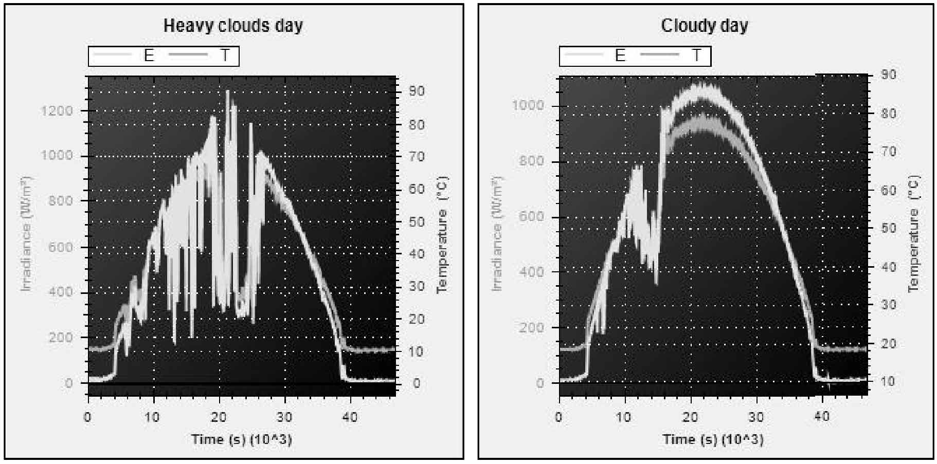
The efficiency of MPPT is affected by various factors, due to the many limitations of MPPT itself. The intensity of light, temperature, cloud thickness, shadow area, illumination angle, weather conditions, and other factors within a day all affect the measurement and calculation of MPPT efficiency. Based on this, MPPT algorithm can be further divided into static MPPT algorithm and dynamic MPPT algorithm. For the static MPPT algorithm, as it is in a static process, it is not necessary to consider the influence of external environment on solar inverters. Therefore, the processing of the static MPPT algorithm in the solar inverter industry is basically at a high level, and its tracking efficiency is basically close to 100%. However, in actual production and application, the static MPPT algorithm will greatly reduce the inverter effect. Therefore, the static MPPT algorithm can only serve as a theoretical basis or support for the dynamic MPPT algorithm. For the overall performance of a solar inverter, it is necessary to pay attention to and measure its dynamic MPPT efficiency. The testing process of dynamic MPPT efficiency needs to consider various limiting factors. Taking the weather conditions within a day as an example, simulate the conditions such as light intensity and temperature within a day, set the measurement time as 24 hours under the simulated conditions, and use a photovoltaic simulator to simulate the dynamic changes in the output of the photovoltaic array over time. The photovoltaic simulator used in this article is AMETEK ETS1000, which has an authoritative position among various photovoltaic simulators due to its advantages of providing various external conditions such as sunny, cloudy, and cloudy days, customizable weather conditions, free external environment matching, setting test duration, and programmable output DC power supply. The simulated irradiance and temperature changes under cloudy and cloudy conditions are shown in Figure 1.
In addition, when measuring the efficiency of dynamic MPPT, it is necessary to avoid the supply power error caused by the algorithm of the photovoltaic simulator itself. When simulating the IV curve, AMETEK ETS1000 can interpolate 128 times per second, which is currently the most linearly changing IV curve given by all photovoltaic simulators.
The most important aspect of measuring the efficiency of dynamic MPPT is the calculation of the tracking accuracy of the photovoltaic simulator MPPT. The calculation method is that the simulator collects the output voltage and output current values at the current time, multiplies them to obtain the output power value at the current time, and then divides them by the maximum power value of the IV curve at the current time. It is necessary to avoid the problem of supply power error introduced by the algorithm of the photovoltaic simulator itself here, because the output voltage and output current values in MPPT accuracy calculation need to be collected in real time and have a certain measurement time window. Taking 20ms as an example, when the IV curve is linearly interpolated at high speed, it can be executed 128 times per second, about 7.8ms once. Therefore, within the 20ms time window, the IV curve changes twice, The maximum power value divided by the simulator after the first collection of output voltage and output current is the maximum power value after the second IV curve change, which brings certain errors to the MPPT calculation.
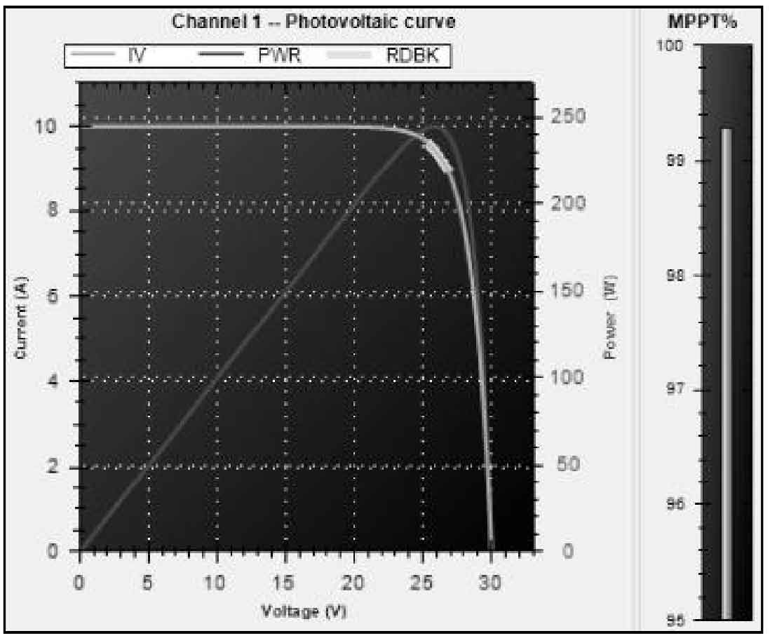
To improve the authenticity of dynamic MPPT efficiency, it is necessary to match appropriate IV curve update rates and time measurement windows. Taking the time window of 20ms as an example, when the IV curve is set to update every 100ms, output power read back is performed to ensure that the current output power measurement value and the update of the IV curve are synchronized and matched in real-time. On this basis, AMETEK ETS1000 provides a visual dynamic MPPT efficiency measurement window, as shown in Figure 2.
2.2 Overall efficiency testing of solar inverters
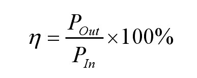
For the testing of the overall efficiency of solar inverters, it is necessary to simultaneously measure the input DC voltage and DC current values of the solar inverter, as well as the output AC voltage and AC current values of the solar inverter when the solar inverter is in stable operating output. The calculation formula is as follows:
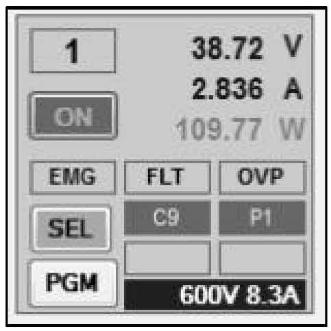
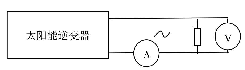
Through the visualization interface of the photovoltaic inverter simulator, the DC voltage and current values at the input end of the DC power supply can be accurately obtained, as shown in Figure 3. The current input DC voltage is 38.72V, DC current is 2.836A, and input power is 109.77W. To protect the circuit, a power resistor is connected in parallel at the AC output end of the solar inverter, an AC voltmeter is connected in parallel at the power resistor, and the AC ammeter is connected in series to the positive end of the AC output. The schematic diagram is shown in Figure 4.