
I have designed and evaluated a two-stage non-isolated solar inverter for distributed photovoltaic generation. The central objective is to combine a dual-input Boost stage, an H6 bridge inverter, dual-core digital control, and wireless monitoring in a compact solar inverter that can be deployed in residential and small commercial environments. The architecture is intended to improve energy yield, reduce common-mode leakage current, and provide data visibility without increasing the cost of the solar inverter platform. I use first-person engineering reasoning throughout: I first define the power-stage behavior, then derive the control laws, then describe the hardware and software partitioning, and finally compare simulation and experimental results.
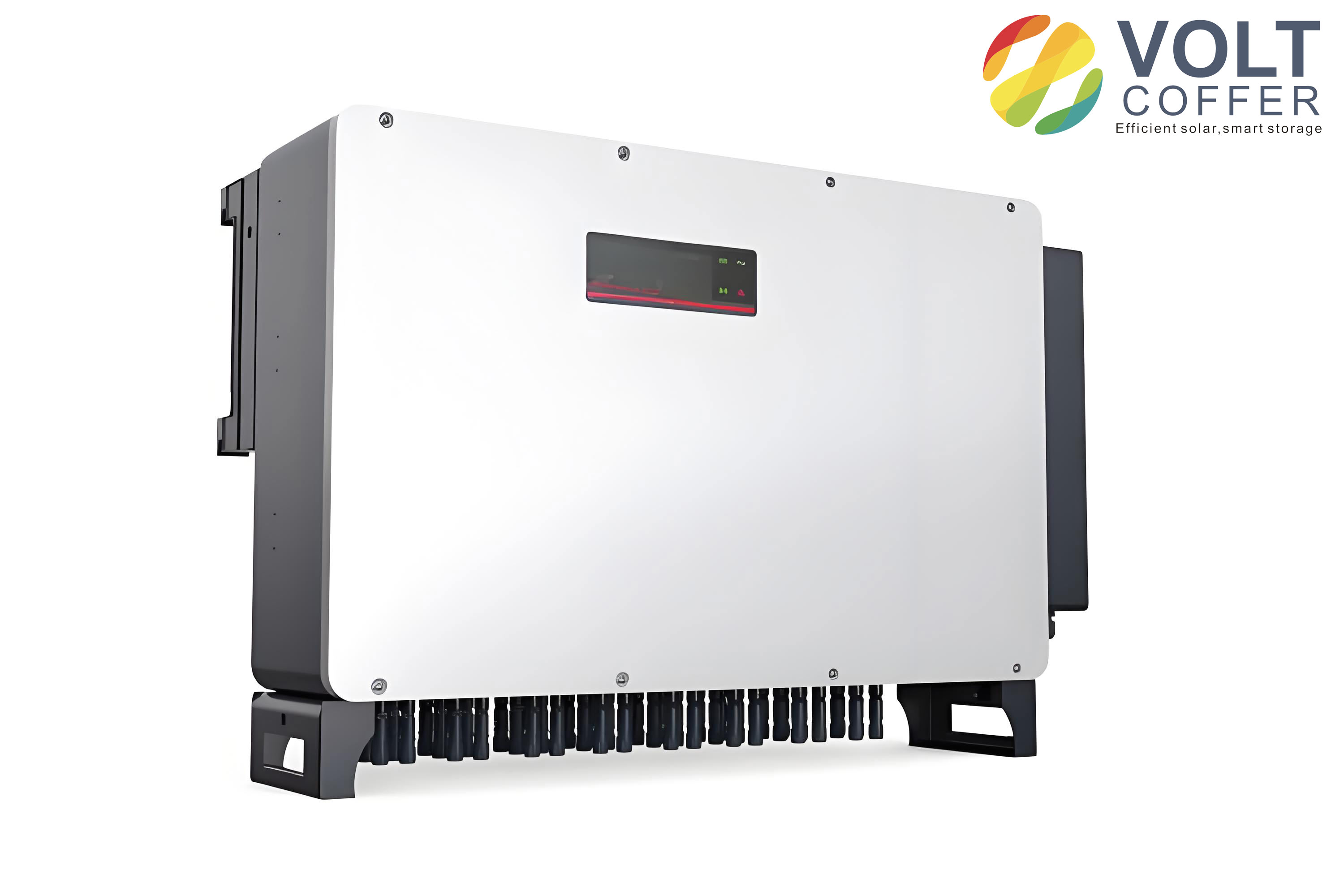
Motivation for a Distributed Solar Inverter
Distributed photovoltaic generation differs from centralized plant generation because the source is dispersed, the power level is lower, and the installation environment is less controlled. A residential solar inverter must therefore tolerate wide input-voltage variation, partial shading, grid-voltage fluctuation, and long periods of low irradiance. I chose a dual-input Boost stage so that two photovoltaic strings can operate independently. This choice reduces current stress in each Boost branch, improves shading tolerance, and allows the same solar inverter to process a higher total power without increasing the current rating of every semiconductor. The H6 bridge is selected because it suppresses common-mode leakage current while retaining the high efficiency of a transformerless solar inverter.
I organize the design around four requirements. First, the solar inverter must track the maximum power point of each input. Second, it must deliver a sinusoidal current synchronized with the grid. Third, it must limit leakage current through the photovoltaic parasitic capacitance. Fourth, it must report operating data to a local or remote monitoring system. These requirements shape the topology, the modulation scheme, and the control partition.
| Requirement | Design choice | Expected benefit |
|---|---|---|
| Wide input voltage | Two independent Boost converters | Independent maximum power point tracking and reduced current stress |
| Low leakage current | H6 bridge topology | Stable common-mode voltage and reduced leakage current |
| Fast digital control | Dual-core DSP partition | Independent front-end and grid-side control |
| Remote visibility | Wi-Fi and serial protocol | Real-time monitoring of the solar inverter |
Overall Power Architecture
The power stage of the solar inverter is a two-stage structure. The first stage converts the photovoltaic input into a regulated DC bus. The second stage converts the DC bus into grid current. I define the main bus voltage as \(V_{bus}\), the first input as \(V_{pv1}\), the second input as \(V_{pv2}\), and the grid voltage as \(v_g(t)\). The bus voltage is controlled at approximately 400 V in the nominal two-stage mode. When the photovoltaic open-circuit voltage is already high enough, the Boost stage can be bypassed and the system operates in a single-stage manner. This mode transition reduces switching losses when the input voltage is high.
$$V_{bus}=400\text{ V}\quad \text{for nominal two-stage operation}$$
$$V_{bus}\approx V_{pv}\quad \text{when the Boost stage is bypassed}$$
I use two input branches because the total rated power is 5 kW and the maximum single-branch power is 3 kW. Each branch has its own inductor, switch, diode, current sensor, and voltage sensor. The branches share the DC bus, the H6 bridge, the output filter, and the grid interface. This shared output stage minimizes size and cost while preserving independent input control.
| Parameter | Symbol | Value | Unit |
|---|---|---|---|
| Maximum single-branch power | \(P_{pv,max}\) | 3000 | W |
| Rated single-branch power | \(P_{pv,rated}\) | 2500 | W |
| Input voltage range | \(V_{pv}\) | 150-500 | V |
| Maximum power point range | \(V_{mpp}\) | 250-500 | V |
| Maximum input current | \(I_{pv,max}\) | 15 | A |
| Input overvoltage protection | \(V_{pv,ov}\) | 550 | V |
| Grid voltage | \(V_{g}\) | 230 | V |
| Grid frequency | \(f_g\) | 50 | Hz |
| Maximum AC current | \(I_{ac,max}\) | 25 | A |
| Maximum efficiency | \(\eta_{max}\) | 95 | % |
| Leakage current protection | \(I_{leak,prot}\) | 20 | mA |
Dual Boost Stage and Operating Modes
The Boost stage is responsible for voltage elevation and maximum power point tracking. I analyze each branch as a conventional Boost converter. The steady-state voltage ratio is
$$\frac{V_{bus}}{V_{pv}}=\frac{1}{1-D}$$
where \(D\) is the duty cycle. The inductor current can operate in discontinuous conduction mode or continuous conduction mode. I define a mode transition at approximately 600 W per branch. Below this power, the branch operates in discontinuous conduction mode, which can reduce switching losses and diode reverse-recovery effects. Above this power, the branch operates in continuous conduction mode, which reduces current ripple and improves the utilization of the semiconductor devices.
$$L>\frac{V_{pv,min}D_{max}}{\Delta I f_s}$$
$$D_{max}=1-\frac{V_{pv,min}}{V_{bus}}=1-\frac{150}{400}=0.625$$
For the selected switching frequency of 20 kHz, the inductor must be large enough to maintain continuous current at the desired power level. I selected an inductance in the range of approximately 0.57 mH to 2.35 mH after considering the maximum and minimum input voltages. A practical value near 1.97 mH was chosen for the nominal maximum power point voltage. The bus capacitor is sized to limit voltage ripple and to provide the instantaneous energy buffer between the Boost stage and the H6 bridge.
$$C_{bus}>\frac{P_{rated}}{\omega V_{bus}\Delta V_{bus}}$$
$$C_{bus}>\frac{5000}{2\pi\cdot 50\cdot 400\cdot 20}\approx 1990\ \mu F$$
I implemented the bus capacitance using series and parallel combinations to obtain approximately 2000 \(\mu F\) with a voltage rating above the maximum bus voltage. This provides margin against grid-frequency ripple and transient load changes. The dual Boost stage can be configured in three control modes: dual constant-voltage mode, one-branch maximum power point tracking plus one-branch constant-voltage mode, and dual maximum power point tracking mode.
| Mode | Branch 1 control | Branch 2 control | Typical use |
|---|---|---|---|
| Dual constant-voltage | Constant voltage | Constant voltage | Uniform irradiance and stable conditions |
| Single maximum power point tracking | Maximum power point tracking | Constant voltage | One shaded string and one unshaded string |
| Dual maximum power point tracking | Maximum power point tracking | Maximum power point tracking | Independent strings and changing irradiance |
The dual maximum power point tracking mode is the most flexible because each branch searches for its own maximum power point. The constant-voltage mode is useful when the photovoltaic source has a known and stable maximum power point voltage ratio. I also use a global scan function to handle multi-peak power-voltage curves caused by partial shading. The scan range is set between approximately 0.4 and 0.8 of the open-circuit voltage.
$$V_{start}=0.8V_{oc}$$
$$V_{scan}\in[0.4V_{oc},0.8V_{oc}]$$
Photovoltaic Source Model
For simulation and control development, I use the single-diode model and an engineering approximation. The single-diode model is
$$I=I_{ph}-I_0\left[\exp\left(\frac{q(V+IR_s)}{AKT}\right)-1\right]-\frac{V+IR_s}{R_{sh}}$$
where \(I_{ph}\) is the photocurrent, \(I_0\) is the diode saturation current, \(q\) is the electron charge, \(A\) is the diode ideality factor, \(K\) is Boltzmann’s constant, \(T\) is temperature, \(R_s\) is series resistance, and \(R_{sh}\) is shunt resistance. The engineering model uses the short-circuit current, open-circuit voltage, maximum power current, and maximum power voltage at a reference irradiance and temperature.
$$I_{sc}=I_{sc,ref}\left(1+\frac{S}{S_{ref}}a\Delta T\right)$$
$$V_{oc}=V_{oc,ref}\left(1+\frac{S}{S_{ref}}b\Delta S+c\Delta T\right)$$
$$I_m=I_{m,ref}\left(1+\frac{S}{S_{ref}}a\Delta T\right)$$
$$V_m=V_{m,ref}\left(1+\frac{S}{S_{ref}}b\Delta S+c\Delta T\right)$$
I use these equations in a simulation model to represent a string of eight modules. The single string has an open-circuit voltage near 375 V, a short-circuit current near 11 A, and a maximum power near 2880 W under the reference condition. This matches the intended 3 kW branch rating with margin for losses and environmental variation.
| Parameter | Single module | String of eight modules |
|---|---|---|
| Short-circuit current | 10.9 A | 10.9 A |
| Open-circuit voltage | 48 V | 375 V |
| Maximum power current | 9.9 A | 9.9 A |
| Maximum power voltage | 36 V | 288 V |
| Maximum power | 360 W | 2880 W |
H6 Bridge Solar Inverter
The second stage is an H6 bridge solar inverter. It contains six switches, two freewheeling diodes, and an output filter. The high-frequency switches generate a sinusoidal pulse-width modulation pattern, while the two low-frequency switches perform grid-frequency commutation. The major advantage of the H6 bridge is that it maintains a nearly constant common-mode voltage during switching transitions. This reduces the leakage current that flows through the parasitic capacitance between the photovoltaic array and ground.
I define the bridge midpoint voltages as \(U_{AN}\) and \(U_{BN}\). The common-mode voltage is
$$U_{cm}=\frac{1}{2}(U_{AN}+U_{BN})$$
The leakage current through the parasitic capacitance \(C_{pv}\) is
$$i_{cm}=C_{pv}\frac{dU_{cm}}{dt}$$
When the common-mode voltage is nearly constant, the derivative is small, and the leakage current is suppressed. The H6 bridge has four main operating states in each grid cycle.
| State | Conducting devices | Bridge voltage \(U_{AB}\) | Common-mode behavior |
|---|---|---|---|
| Positive active | High-frequency switch pair and positive freewheel switch | \(+V_{bus}\) | Common-mode voltage stable |
| Positive freewheel | Positive freewheel switch only | \(0\) | Common-mode voltage stable |
| Negative active | High-frequency switch pair and negative freewheel switch | \(-V_{bus}\) | Common-mode voltage stable |
| Negative freewheel | Negative freewheel switch only | \(0\) | Common-mode voltage stable |
For current control, I model the H6 bridge as a single-phase inverter with an LCL output filter. The grid is treated as a stiff voltage source for current-loop design. The output current \(i_g\) is controlled to follow a reference \(i_g^*\). The state equation during active conduction is
$$V_{bus}=L_1\frac{di_1}{dt}+L_2\frac{di_g}{dt}+Ri_g+v_g$$
Assuming a symmetrical LCL filter with \(L_1=L_2=L\), this becomes
$$V_{bus}=2L\frac{di_g}{dt}+Ri_g+v_g$$
The deadbeat current controller calculates the duty cycle that forces the current to reach its reference in one sampling interval. The discrete-time equation is
$$D(k)=\frac{V_{bus}(k)+Ri_g(k)+\frac{2L}{T_s}\left[i_g^*(k+1)-i_g(k)\right]}{V_{bus}(k)}$$
This controller provides fast tracking and good dynamic response. I combine it with a phase-locked loop so that the grid current remains synchronized with the grid voltage. The current reference is derived from the bus voltage control loop and the grid phase angle.
$$i_g^*(t)=I_m\sin(\theta_g)$$
$$\theta_g=2\pi f_g t+\phi_g$$
Dual-Core Control Partition
I partition the control system into two digital signal processors. The first processor controls the dual Boost stage, performs maximum power point tracking, manages the state machine, and handles monitoring communication. The second processor controls the H6 bridge, performs grid current regulation, executes the deadbeat algorithm, and monitors grid conditions. This partition reduces the computational burden on each processor and allows the front-end and grid-side control loops to run independently.
The two processors exchange status and fault information through general-purpose input/output pins. I define a simple synchronization protocol with five pins. Two pins carry the front-end state, and three pins carry the grid-side state and fault category. This allows each processor to verify the readiness of the other before entering a new operating mode.
| Processor | Pin | Direction | Function |
|---|---|---|---|
| Front-end DSP | GPIO28 | Output | Front-end ready or tracking state |
| Front-end DSP | GPIO26 | Output | Bus voltage ready or maximum power point tracking active |
| Front-end DSP | GPIO31 | Input | Grid-side fault or ready state |
| Front-end DSP | GPIO30 | Input | Grid-side fault or ready state |
| Front-end DSP | GPIO27 | Input | Grid-side fault or ready state |
| Grid-side DSP | GPIO31 | Output | Grid-side ready or fault category |
| Grid-side DSP | GPIO30 | Output | Grid-side ready or fault category |
| Grid-side DSP | GPIO27 | Output | Grid-side ready or fault category |
| Grid-side DSP | GPIO28 | Input | Front-end ready or tracking state |
| Grid-side DSP | GPIO26 | Input | Front-end ready or tracking state |
I also implement a state machine that governs the solar inverter from startup to shutdown. The states are waiting, checking, normal, fault, and reconnect. This state machine prevents the solar inverter from connecting to the grid before the input voltage, bus voltage, grid voltage, and grid frequency are within valid ranges. It also ensures that a fault immediately disables the power stage and opens the grid relay.
| State | Entry condition | Action | Exit condition |
|---|---|---|---|
| Waiting | Input voltage above start threshold but below operating threshold | Keep power stage off | Input voltage reaches operating range |
| Checking | Input voltage valid | Measure grid and bus, soft-start Boost, regulate bus | All checks pass for the validation interval |
| Normal | Bus and grid valid | Run maximum power point tracking and grid current control | Fault or loss of grid |
| Fault | Any protection trip | Disable drivers, open relay, display fault | Fault cleared and safe condition detected |
| Reconnect | Fault cleared | Repeat validation and soft start | Validation passes |
Maximum Power Point Tracking Control
I use a perturb-and-observe method with a global scan option. The algorithm samples the photovoltaic voltage and current, computes power, and perturbs the operating voltage in the direction that increases power. The power change and voltage change are
$$\Delta P=P(k)-P(k-1)$$
$$\Delta V=V(k)-V(k-1)$$
If \(\Delta P/\Delta V>0\), I move the operating voltage in the same direction. If \(\Delta P/\Delta V<0\), I reverse the direction. When the power change falls below a threshold, the algorithm enters a steady state and holds the operating point. A global scan is executed periodically to detect multiple peaks caused by partial shading.
$$\left|\frac{\Delta P}{\Delta V}\right|<\varepsilon \Rightarrow \text{steady state}$$
I tested the MPPT behavior with a photovoltaic simulator. The measured tracking efficiency remained above 99% across several power levels from 500 W to 3000 W. The front-end Boost stage was able to reach the maximum power point quickly and maintain stable operation. The dual-branch structure allowed each branch to track independently, which is important when one string is shaded and the other is not.
| Test power | Tracking behavior | Tracking efficiency |
|---|---|---|
| 500 W | Fast convergence, stable operation | >99% |
| 1000 W | Fast convergence, stable operation | >99% |
| 1500 W | Fast convergence, stable operation | >99% |
| 2000 W | Fast convergence, stable operation | >99% |
| 2500 W | Fast convergence, stable operation | >99% |
| 3000 W | Fast convergence, stable operation | >99% |
Grid Current Control and Deadbeat Algorithm
The grid-side control loop uses a voltage outer loop and a current inner loop. The voltage outer loop regulates the DC bus and generates the current amplitude reference. The current inner loop uses the deadbeat controller to force the grid current to its reference. The deadbeat controller is derived from the discrete-time model of the output filter.
$$i_g(k+1)=i_g(k)+\frac{T_s}{2L}\left[V_{bus}D(k)-v_g(k)-Ri_g(k)\right]$$
Solving for \(D(k)\) gives the control law used in the digital signal processor. The controller is computationally simple and provides a fast transient response. I combine it with a phase-locked loop to ensure that the current reference is synchronized with the grid voltage. The phase-locked loop detects the zero crossings of the grid voltage and estimates the frequency and phase.
$$\theta_g(k+1)=\theta_g(k)+2\pi f_g T_s$$
$$i_g^*(k)=I_m\sin(\theta_g(k))$$
The output filter is an LCL filter. I selected the filter components so that the resonant frequency is well below the switching frequency and well above the grid frequency. This attenuates switching harmonics while maintaining a small filter size.
$$f_{res}=\frac{1}{2\pi}\sqrt{\frac{L_1+L_2}{L_1L_2C_f}}$$
$$10f_g<f_{res}<0.5f_s$$
For a 20 kHz switching frequency and a 50 Hz grid frequency, the resonant frequency is placed near 2 kHz. The inverter-side and grid-side inductances are approximately 0.97 mH each, and the filter capacitance is approximately 4.7 \(\mu F\).
| Filter parameter | Symbol | Value |
|---|---|---|
| Inverter-side inductance | \(L_1\) | 0.97 mH |
| Grid-side inductance | \(L_2\) | 0.97 mH |
| Filter capacitance | \(C_f\) | 4.7 \(\mu F\) |
| Switching frequency | \(f_s\) | 20 kHz |
| Grid frequency | \(f_g\) | 50 Hz |
| Resonant frequency | \(f_{res}\) | approximately 2 kHz |
Modulation and Switching Logic
The H6 bridge uses unipolar sinusoidal pulse-width modulation. The high-frequency switches are driven by complementary signals during each half-cycle, while the low-frequency switches change state at the grid frequency. The switching logic prevents the freewheeling path from being interrupted and maintains a stable common-mode voltage.
I define the high-frequency control signals as \(S_1\) and \(S_2\), and the grid-frequency signals as \(S_5\) and \(S_6\). The actual gate signals are
$$G_1=S_1\cdot S_5$$
$$G_4=S_1\cdot S_5$$
$$G_2=S_2\cdot S_6$$
$$G_3=S_2\cdot S_6$$
$$G_5=S_5$$
$$G_6=S_6$$
This logic ensures that the active switches and the freewheeling switches are coordinated. The result is a bridge voltage that alternates between \(+V_{bus}\), \(0\), and \(-V_{bus}\) while the common-mode voltage remains nearly constant.
| Grid half-cycle | High-frequency active pair | Freewheeling switch | Bridge voltage |
|---|---|---|---|
| Positive | \(Q_1,Q_4\) | \(Q_5\) | \(+V_{bus}\) or 0 |
| Negative | \(Q_2,Q_3\) | \(Q_6\) | \(-V_{bus}\) or 0 |
Hardware Design and Component Selection
I selected the power semiconductors to withstand the maximum bus voltage and current. The Boost switch and diode must tolerate 600 V or more. I used a 600 V insulated-gate bipolar transistor with a current rating above 40 A for each Boost branch. The H6 bridge uses similar devices to simplify procurement and reduce the number of unique components. The output filter inductors are designed for the rated current and the desired ripple current.
The auxiliary power supply is a flyback converter based on an integrated controller with an internal high-voltage switch. It accepts the DC bus voltage and provides regulated rails for the control boards, gate drivers, sensors, and relays. I designed the flyback transformer with multiple secondary windings to supply \(+15 V\), \(-15 V\), \(+12 V\), \(+9 V\), and isolated gate-drive voltages.
$$N_1=110\text{ turns}$$
$$N_0=11\text{ turns}$$
$$N_1/N_2=12.5,\quad N_1/N_3=16.7,\quad N_1/N_4=12.5$$
| Auxiliary rail | Voltage | Load |
|---|---|---|
| Control analog positive | +15 V | Sensors and operational amplifiers |
| Control analog negative | -15 V | Signal conditioning |
| Gate-drive rail | +12 V | Isolated drivers |
| Relay rail | +9 V | Grid relay |
| Isolated gate rails | Multiple | H6 bridge high-side and low-side drivers |
Signal Sampling and Protection
I designed sensing circuits for the photovoltaic voltage and current, bus voltage, grid voltage, grid current, and heat-sink temperature. The photovoltaic voltage is scaled with a high-impedance resistor divider. The photovoltaic current is measured with a Hall-effect sensor. The grid voltage is scaled and level-shifted to match the analog-to-digital converter range. The grid current is measured with a current transducer and converted to a unipolar signal for the processor.
$$V_{adc}=k_v V_{pv}$$
$$V_{adc}=k_i I_{pv}$$
The protection functions include input overvoltage, input overcurrent, bus overvoltage, bus undervoltage, grid overvoltage, grid undervoltage, grid overfrequency, grid underfrequency, output overcurrent, leakage current, and over-temperature. Hardware comparators provide fast protection independent of software. Software protection provides additional logic and fault classification.
| Protection | Threshold | Action |
|---|---|---|
| Input overvoltage | 550 V | Stop Boost, open relay |
| Input overcurrent | Per-branch limit | Disable Boost driver |
| Bus overvoltage | 550 V | Disable inverter, open relay |
| Bus undervoltage | 350 V | Stop grid connection |
| Grid overvoltage | 264 V | Open relay |
| Grid undervoltage | 210 V | Open relay |
| Grid overfrequency | 50.5 Hz | Open relay |
| Grid underfrequency | 49.3 Hz | Open relay |
| Leakage current | 20 mA | Disable inverter |
| Over-temperature | Heat-sink limit | Derate or stop |
Communication and Data Monitoring
The solar inverter includes a wireless monitoring module. I use a serial-to-Wi-Fi module that presents a transparent serial interface to the first processor. The processor formats data using a Modbus-like protocol with a preamble, address, function code, length, data field, CRC, and end byte. The CRC improves data integrity in the presence of electromagnetic noise.
| Field | Description |
|---|---|
| Preamble | Start of frame |
| Address | Unique identifier of the solar inverter |
| Function code | Read or write command |
| Length | Number of data bytes |
| Data | Voltage, current, power, status, or settings |
| CRC | Cyclic redundancy check |
| End byte | End of frame |
I implemented command tables for reading and writing. The read commands include grid current, operating state, photovoltaic voltage and current, input power, output power, daily energy, grid voltage, grid frequency, and fault status. The write commands include protection thresholds, time reset, energy counter reset, and control-mode selection.
$$CRC=f_{crc}(data)$$
The monitoring data is transmitted once per second. A host computer can display the data and log it for later analysis. This makes the solar inverter a connected device rather than a stand-alone power converter. The wireless link also allows a cluster of solar inverter units to be monitored from a single point.
Simulation Verification
I used simulation to verify the photovoltaic model, the dual Boost stage, the H6 bridge, and the deadbeat current controller. The photovoltaic model produced the expected single-peak power-voltage curve under uniform irradiance and multi-peak behavior under partial shading. The perturb-and-observe algorithm converged to the maximum power point with small steady-state oscillation. The deadbeat controller tracked the current reference with low harmonic distortion.
| Simulation case | Reference | Result |
|---|---|---|
| Photovoltaic string | 8 modules in series | Open-circuit voltage near 375 V, maximum power near 2880 W |
| Maximum power point tracking | 500 W to 3000 W | Convergence to maximum power point with stable operation |
| Deadbeat current control | 7 A, 14 A, 10 A, 3 A steps | Fast tracking and low transient distortion |
| Common-mode voltage | 400 V bus | Stable common-mode voltage and leakage current below 10 mA |
The simulated grid current showed a total harmonic distortion below 1.5% under steady conditions. During power steps, the current recovered quickly and the distortion remained low. The common-mode current simulation showed that the H6 bridge limits leakage current to a safe level.
$$THD=\frac{\sqrt{\sum_{h=2}^{H}I_h^2}}{I_1}\times 100\%$$
Experimental Setup
I built a prototype of the dual-Boost H6 solar inverter and tested it with a programmable DC source, a photovoltaic simulator, a power analyzer, a digital oscilloscope, current probes, and a host computer. The prototype includes the main power board, the dual-core control board, the auxiliary power supply, the gate-drive circuits, the sensors, and the wireless module.
| Equipment | Purpose |
|---|---|
| Photovoltaic simulator | Emulate photovoltaic strings under different irradiance and temperature |
| Programmable DC source | Provide controlled input voltage and current |
| Power analyzer | Measure AC power, efficiency, and harmonic distortion |
| Digital oscilloscope | Observe gate signals, inductor current, and grid current |
| Current probe | Measure Boost inductor current and leakage current |
| Host computer | Receive monitoring data and display operating status |
Experimental Results
The auxiliary power supply operated correctly from the DC bus and provided stable rails. The measured output voltages were close to the design values. The switch drain-source voltage remained below the device rating, and the snubber and clamp circuits limited the turn-off spike. The gate-drive waveforms for the Boost stage and the H6 bridge matched the expected logic.
| Measurement | Observed value | Design target |
|---|---|---|
| Auxiliary positive rail | 15.4 V | 15 V |
| Auxiliary negative rail | -12.9 V | -12 V |
| Gate-drive rail | 11.1 V | 12 V |
| Relay rail | 7.68 V | 9 V |
| Boost switching frequency | 20 kHz | 20 kHz |
| H6 high-frequency switching | 20 kHz | 20 kHz |
| H6 grid-frequency switching | 50 Hz | 50 Hz |
The Boost stage produced a smooth soft-start. The bus voltage rose from the input voltage to 400 V without overshoot. The transition between discontinuous and continuous conduction modes occurred near the expected power level. The inductor current changed from a triangular discontinuous waveform to a continuous waveform as the load increased. This confirms that the selected inductance is appropriate for the power range.
| Operating power | Inductor current mode | Observation |
|---|---|---|
| 367.7 W | Discontinuous | Current returns to zero each switching cycle |
| 697.5 W | Boundary | Current touches zero at the switching instant |
| 906.3 W | Continuous | Current remains above zero |
The maximum power point tracking tests were performed at 500 W, 1000 W, 1500 W, 2000 W, 2500 W, and 3000 W. The front-end converters tracked the maximum power point in each case. The tracking speed was fast enough to follow slowly changing irradiance. The dual-branch operation allowed both inputs to operate independently. The measured tracking efficiency was above 99% at all tested power levels.
| Test power | Tracking efficiency | Steady-state behavior |
|---|---|---|
| 500 W | >99% | Stable with low oscillation |
| 1000 W | >99% | Stable with low oscillation |
| 1500 W | >99% | Stable with low oscillation |
| 2000 W | >99% | Stable with low oscillation |
| 2500 W | >99% | Stable with low oscillation |
| 3000 W | >99% | Stable with low oscillation |
The grid-connected tests showed that the solar inverter delivered a sinusoidal current synchronized with the grid voltage. The current total harmonic distortion decreased as power increased. At 2000 W and above, the total harmonic distortion was below 3%. The conversion efficiency increased with power and reached approximately 96% at 2000 W and 3000 W. The Boost switch temperature remained below the thermal limit at full power.
| Input power | Boost switch temperature | Efficiency | Grid current quality |
|---|---|---|---|
| 800 W | 30.2 °C | 94% | Sinusoidal, moderate distortion |
| 1200 W | 33.0 °C | 94% | Sinusoidal, moderate distortion |
| 2000 W | 44.9 °C | 96% | Sinusoidal, low distortion |
| 3000 W | 68.7 °C | 96% | Sinusoidal, low distortion |
I measured the common-mode voltage and leakage current to verify the H6 bridge behavior. The common-mode voltage switched in a controlled manner around the bus voltage, and the leakage current remained below the protection threshold. At 500 W and 3000 W, the leakage current stayed within a safe range. The measured root-mean-square value of the leakage current sensing signal changed by less than 20 mV, which corresponds to less than 20 mA of leakage current. This confirms that the H6 bridge suppresses common-mode leakage current effectively.
| Condition | Common-mode voltage | Leakage current |
|---|---|---|
| 500 W | Controlled switching around bus voltage | Below protection threshold |
| 3000 W | Controlled switching around bus voltage | Below protection threshold |
Data Monitoring Results
The liquid-crystal display showed the operating state, input voltage, input current, output power, daily energy, grid voltage, grid frequency, and fault messages. The display updated smoothly and the button interface allowed the user to switch pages. The wireless module transmitted the monitoring data to the host computer. The host computer displayed the received values and stored them for analysis. The communication worked once per second, which is sufficient for residential monitoring.
| Display item | Example content | Update behavior |
|---|---|---|
| Operating state | Waiting, checking, normal, fault, reconnect | On state change |
| Input voltage | Photovoltaic voltage | Periodic |
| Input current | Photovoltaic current | Periodic |
| Output power | AC power | Periodic |
| Daily energy | Accumulated energy | Periodic |
| Grid voltage | AC voltage | Periodic |
| Grid frequency | AC frequency | Periodic |
| Fault message | Specific fault type | On fault |
Discussion
The dual-Boost H6 solar inverter meets the intended goals of high input flexibility, low leakage current, and digital connectivity. The dual Boost stage allows independent maximum power point tracking and reduces current stress. The H6 bridge provides a low-leakage transformerless interface. The dual-core control partition improves computational margin and simplifies the separation of front-end and grid-side functions. The wireless monitoring link makes the solar inverter suitable for distributed energy management.
The main trade-off is the increased component count in the power stage. The second Boost branch adds an inductor, a switch, a diode, and sensing circuitry. However, the shared H6 bridge and output filter offset this cost. The H6 bridge also requires a more complex gate-drive arrangement than a conventional H4 bridge, but the leakage-current benefit is significant for non-isolated solar inverter applications.
| Design aspect | Benefit | Trade-off |
|---|---|---|
| Dual Boost input | Independent tracking and lower current stress | Additional inductor and switch |
| H6 bridge | Low leakage current | More complex drive logic |
| Dual-core DSP | Independent control loops | Inter-processor synchronization |
| Wireless monitoring | Remote visibility | Additional communication hardware |
Further Work
I will extend the control design in several directions. First, I will add a fuzzy or adaptive gain to the deadbeat current controller to improve robustness under weak-grid conditions. Second, I will develop a more accurate global scan method for partial shading that does not disturb the grid current. Third, I will implement an islanding detection function and validate it according to relevant grid-connection standards. Fourth, I will optimize the thermal design and electromagnetic compatibility of the solar inverter for higher ambient temperatures.
I will also improve the monitoring system. A cloud-connected data service could aggregate measurements from multiple solar inverter units and provide fault prediction. The data could be used to estimate degradation, detect shading patterns, and schedule maintenance. This would turn the solar inverter into an intelligent energy node rather than a simple power converter.
$$P_{loss}=P_{dc}-P_{ac}$$
$$\eta=\frac{P_{ac}}{P_{dc}}\times 100\%$$
Conclusion
I designed, simulated, built, and tested a dual-Boost H6 solar inverter for distributed photovoltaic generation. The power stage uses two independent Boost branches and a shared H6 bridge. The control system uses two digital signal processors: one for front-end maximum power point tracking and one for grid-side current control. The modulation scheme and H6 topology reduce common-mode leakage current. The deadbeat current controller provides fast grid-current tracking. The wireless module enables remote monitoring.
The experimental results confirm that the solar inverter can track the maximum power point with high efficiency, deliver low-distortion grid current, and maintain leakage current within safe limits. The dual-core control partition and the modular hardware design provide a practical basis for future product development. I conclude that the proposed architecture is a viable solution for a compact, efficient, and connected solar inverter in distributed photovoltaic systems.
</f_{res}