
In modern power systems, the grid connected inverter plays a pivotal role in integrating renewable energy sources and ensuring power quality. As a critical interface between distributed generation and the grid, the performance of a grid connected inverter directly impacts grid stability and efficiency. Therefore, enhancing control precision and reducing output current ripple have been central focuses in the development of control strategies for grid connected inverters. Traditional methods, such as repetitive control and proportional-resonant control, have been employed to address these issues. For instance, a repetitive-proportional resonant controller has been proposed to mitigate current ripple and harmonic content in grid connected inverters. However, these approaches often involve complex parameter tuning and may lack rapid dynamic response. In recent years, model predictive current control (MPCC) has gained widespread adoption in power electronics due to its fast response, simplicity, and avoidance of intricate parameter adjustments. MPCC operates by predicting future system states and optimizing control actions through a cost function, making it highly suitable for applications like grid connected inverters.
MPCC for inverters can be categorized based on the number of voltage vectors applied per sampling cycle. The first category is single-vector MPCC, where only one of the eight basic voltage vectors (including two zero vectors) is selected per control period. While straightforward, this method suffers from limited voltage vector direction and magnitude, leading to suboptimal control performance. The second category is dual-vector MPCC, which involves selecting two optimal voltage vectors from the basic set. This approach expands the candidate voltage coverage and can improve steady-state performance. For example, duty-cycle dual-vector MPCC combines an active vector with a zero vector to adjust output voltage magnitude, but the direction remains fixed. Alternatively, a more flexible dual-vector MPCC allows both vectors to be chosen from the eight basic vectors, enhancing voltage selection. However, even this method has limitations: the coverage of expected voltage vectors is still constrained, resulting in significant d-axis and q-axis current ripple, reduced current tracking accuracy, and elevated harmonic content in the grid connected current. These drawbacks necessitate further improvements in MPCC strategies for grid connected inverters.
The third category is three-vector MPCC, which introduces a zero vector alongside two active vectors to broaden the output voltage vector range and reduce current ripple. Initially applied in permanent magnet synchronous motors, three-vector MPCC has demonstrated superior steady-state performance compared to dual-vector methods. For instance, a novel three-vector MPCC selects the first active vector through traversal optimization, determines the second based on sector judgment, and incorporates a zero vector to regulate voltage amplitude. Another variant, double optimization three-vector MPCC, employs two cost function optimizations per control cycle to select the optimal vector combination, enabling fast and accurate reference tracking during load transients while minimizing d-axis and q-axis current ripple. Building on these advancements, this article proposes a double optimization three-vector model predictive current control strategy specifically tailored for grid connected inverters. The aim is to address the shortcomings of dual-vector MPCC by expanding voltage vector coverage, reducing current ripple, and enhancing dynamic response, thereby improving the overall performance of grid connected inverters.
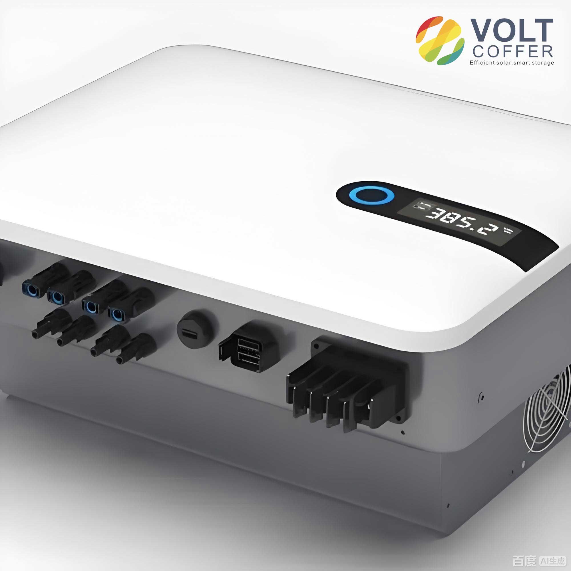
To understand the proposed method, it is essential to first review the dual-vector MPCC for a two-level grid connected inverter. The system comprises a DC voltage source \(V_{dc}\), three-phase grid currents \(i_a\), \(i_b\), \(i_c\), grid voltages \(e_a\), \(e_b\), \(e_c\), filter inductance \(L_s\), and equivalent resistance \(r_s\). In the d-q coordinate system, the discrete-time model of the grid connected inverter is given by:
$$ i_d(k+1) = i_d(k) + \frac{t_s}{L_s} \left( u_d – r_s i_d(k) + \omega L_s i_q(k) – e_d \right) $$
$$ i_q(k+1) = i_q(k) + \frac{t_s}{L_s} \left( u_q – r_s i_q(k) – \omega L_s i_d(k) – e_q \right) $$
where \(i_d(k)\) and \(i_q(k)\) are the sampled currents at time \(k t_s\), \(i_d(k+1)\) and \(i_q(k+1)\) are the predicted currents at \((k+1) t_s\), \(t_s\) is the sampling period, \(u_d\) and \(u_q\) are the inverter output voltages in d-q axes, \(e_d\) and \(e_q\) are the grid voltages in d-q axes, and \(\omega\) is the grid angular frequency. The cost function \(g\) for MPCC is defined as:
$$ g = |i_d^* – i_d(k+1)| + |i_q^* – i_q(k+1)| $$
where \(i_d^*\) and \(i_q^*\) are the reference currents. In dual-vector MPCC, two voltage vectors \(\mathbf{u}_i\) and \(\mathbf{u}_j\) are selected from the seven basic vectors (treating two zero vectors as one) by minimizing \(g\). Their duty times \(t_i\) and \(t_j\) are calculated using the deadbeat principle on the q-axis current, subject to \(t_i + t_j = t_s\). Specifically, the slopes of the d-axis and q-axis currents under different vectors are derived. For a zero vector \(\mathbf{u}_0\), the slopes are:
$$ s_{d0} = \frac{1}{L_s} \left( -e_d – r_s i_d + \omega L_s i_q \right) $$
$$ s_{q0} = \frac{1}{L_s} \left( -e_q – r_s i_q – \omega L_s i_d \right) $$
For active vectors \(\mathbf{u}_i\) and \(\mathbf{u}_j\), the slopes are:
$$ s_{di} = s_{d0} + \frac{u_{di}}{L_s}, \quad s_{qi} = s_{q0} + \frac{u_{qi}}{L_s} $$
$$ s_{dj} = s_{d0} + \frac{u_{dj}}{L_s}, \quad s_{qj} = s_{q0} + \frac{u_{qj}}{L_s} $$
Applying deadbeat control for the q-axis current yields:
$$ i_q(k+1) = i_q(k) + s_{qi} t_i + s_{qj} t_j = i_q^* $$
Solving with \(t_i + t_j = t_s\) gives:
$$ t_i = \frac{i_q^* – i_q(k) – s_{qj} t_s}{s_{qi} – s_{qj}}, \quad t_j = t_s – t_i $$
This process requires 42 current predictions per cycle (since there are 7 choices for the first vector and 6 for the second). However, the voltage vector coverage is limited: when two active vectors are selected, the synthesized vector lies on a line segment between them; when one vector is zero, the coverage is along a ray. This restriction leads to higher current ripple and harmonics in the grid connected inverter output.
To overcome these limitations, the double optimization three-vector MPCC strategy is proposed. It selects three vectors per control cycle: two active vectors and one zero vector, through two cost function optimizations. The key steps include vector selection, duty time calculation with deadbeat control on both d-axis and q-axis currents, time redistribution in case of over-modulation, and vector insertion to modify the switching sequence. This approach significantly expands the voltage vector coverage, reduces current ripple, and improves dynamic response for the grid connected inverter.
The vector selection process in double optimization three-vector MPCC is as follows. First, from the six active voltage vectors, one optimal vector \(\mathbf{u}_i\) is chosen by minimizing the cost function \(g\). Then, from the remaining five active vectors, a second optimal vector \(\mathbf{u}_j\) is selected similarly. Finally, a zero vector \(\mathbf{u}_z\) is included to form the optimal combination. This reduces the number of current predictions to 30 per cycle (6 choices for \(\mathbf{u}_i\) and 5 for \(\mathbf{u}_j\)), lowering computational burden compared to dual-vector MPCC. The coverage area of the expected voltage vector \(\mathbf{u}_d\) becomes a polygon or triangle in the d-q plane, depending on the selected vectors. For example, if \(\mathbf{u}_i\) and \(\mathbf{u}_j\) are adjacent, the coverage is a line segment with the zero vector extending it to a triangle; if they are non-adjacent, the coverage forms a larger polygon. This ensures that the grid connected inverter can output a wider range of voltages, enhancing tracking accuracy.
The duty times for the three vectors are computed using deadbeat control on both d-axis and q-axis currents. The predicted currents are:
$$ i_d(k+1) = i_d(k) + s_{di} t_i + s_{dj} t_j + s_{dz} t_z $$
$$ i_q(k+1) = i_q(k) + s_{qi} t_i + s_{qj} t_j + s_{qz} t_z $$
where \(s_{dz}\) and \(s_{qz}\) are the slopes for the zero vector, and \(t_i\), \(t_j\), \(t_z\) are the duty times with \(t_i + t_j + t_z = t_s\). Setting \(i_d(k+1) = i_d^*\) and \(i_q(k+1) = i_q^*\), and solving the system yields:
$$ t_i = \frac{1}{D} \left[ (e_d – s_{d0}) (s_{qj} – s_{qz}) – (e_q – s_{q0}) (s_{dj} – s_{dz}) + t_s (s_{dj} s_{qz} – s_{dz} s_{qj}) \right] $$
$$ t_j = \frac{1}{D} \left[ (e_q – s_{q0}) (s_{di} – s_{dz}) – (e_d – s_{d0}) (s_{qi} – s_{qz}) + t_s (s_{dz} s_{qi} – s_{di} s_{qz}) \right] $$
$$ t_z = t_s – t_i – t_j $$
where \(D = s_{di} s_{qj} + s_{dj} s_{qz} + s_{dz} s_{qi} – s_{di} s_{qz} – s_{dj} s_{qi} – s_{dz} s_{qj}\). However, in practical scenarios, \(t_i\), \(t_j\), or \(t_z\) may fall outside the range \([0, t_s]\), indicating over-modulation. To handle this, four redistribution cases are defined:
| Case | Condition | Redistribution |
|---|---|---|
| 1 | \(t_i > 0\), \(t_j > 0\), \(t_i + t_j > t_s\) | \(t_i^* = t_i t_s / (t_i + t_j)\), \(t_j^* = t_j t_s / (t_i + t_j)\), \(t_z^* = 0\) |
| 2 | \(t_i < 0\), \(t_j > 0\), \(t_i + t_j < t_s\) | \(t_i^* = 0\), \(t_j^* = t_j\), \(t_z^* = t_s – t_j\) |
| 3 | \(t_i > 0\), \(t_j < 0\), \(t_i + t_j < t_s\) | \(t_i^* = t_i\), \(t_j^* = 0\), \(t_z^* = t_s – t_i\) |
| 4 | \(t_i < 0\), \(t_j < 0\) | \(t_i^* = 0\), \(t_j^* = 0\), \(t_z^* = t_s\) |
After time allocation, vector insertion is applied to modify the switching sequence. Instead of applying vectors in the order \(\mathbf{u}_i\), \(\mathbf{u}_j\), \(\mathbf{u}_z\), the zero vector is inserted at the beginning, middle, and end of the cycle. For example, if \(\mathbf{u}_i = V_1(100)\), \(\mathbf{u}_j = V_2(110)\), and \(\mathbf{u}_z = V_0(000)\) or \(V_7(111)\), the sequence becomes: \(V_0\) for \(t_z/4\), \(V_1\) for \(t_i/2\), \(V_2\) for \(t_j/2\), \(V_7\) for \(t_z/2\), \(V_2\) for \(t_j/2\), \(V_1\) for \(t_i/2\), and \(V_0\) for \(t_z/4\). This reduces switching frequency and current ripple in the grid connected inverter.
To validate the proposed double optimization three-vector MPCC, simulations are conducted in MATLAB/Simulink and compared with dual-vector MPCC and three-vector MPCC. The parameters of the grid connected inverter system are summarized in Table 1.
| Parameter | Value |
|---|---|
| Grid phase voltage peak \(U_e\) | 180 V |
| Grid frequency \(f\) | 50 Hz |
| Filter inductance \(L_s\) | 10 mH |
| Equivalent resistance \(r_s\) | 0.1 Ω |
| DC-link voltage \(V_{dc}\) | 380 V |
| Sampling frequency \(f_s\) | 10 kHz |
| Reference d-axis current \(i_d^*\) | 10 A (steady-state) |
| Reference q-axis current \(i_q^*\) | 0 A |
Steady-state performance is evaluated with \(i_d^* = 10\) A and \(i_q^* = 0\) A. The grid voltages and currents for each method are analyzed. Under dual-vector MPCC, the three-phase currents exhibit noticeable ripple, indicating lower tracking accuracy. Three-vector MPCC reduces this ripple, and double optimization three-vector MPCC further minimizes it, yielding smoother current waveforms. The d-axis and q-axis currents are plotted, showing that the proposed method maintains tighter tracking with reduced fluctuations. To quantify harmonic distortion, fast Fourier transform (FFT) analysis is performed on the output currents. The total harmonic distortion (THD) values are calculated as follows:
$$ \text{THD} = \frac{\sqrt{\sum_{h=2}^{\infty} I_h^2}}{I_1} \times 100\% $$
where \(I_1\) is the fundamental current amplitude and \(I_h\) are harmonic components. The results are compiled in Table 2.
| Control Method | Current THD | Power Factor | d-axis Ripple (A) | q-axis Ripple (A) |
|---|---|---|---|---|
| Dual-vector MPCC | 5.50% | 0.992 | 0.85 | 0.92 |
| Three-vector MPCC | 3.13% | 0.995 | 0.52 | 0.61 |
| Double optimization three-vector MPCC | 1.27% | 0.9994 | 0.18 | 0.21 |
The double optimization three-vector MPCC achieves the lowest THD, highest power factor, and smallest current ripple, demonstrating its superiority in steady-state operation for grid connected inverters. The power factor is computed as:
$$ \text{PF} = \frac{P}{S} = \frac{3 U_e I_1 \cos \phi}{3 U_e I_1} = \cos \phi $$
where \(\phi\) is the phase angle between voltage and current. The proposed method aligns the current closely with the grid voltage, yielding a power factor near unity.
Dynamic performance is tested by step-changing the reference current from 5 A to 10 A at 0.05 s. The response times are measured as the number of control cycles required to settle within 2% of the new reference. Table 3 summarizes the results.
| Control Method | Settling Time (cycles) | Overshoot (%) |
|---|---|---|
| Dual-vector MPCC | 5 | 12.5 |
| Three-vector MPCC | 3 | 8.2 |
| Double optimization three-vector MPCC | 2 | 4.7 |
The proposed method exhibits the fastest settling time and lowest overshoot, highlighting its enhanced dynamic response. This is attributed to the reduced number of predictions (30 vs. 42) and the optimized vector selection, which enable quicker adjustments in the grid connected inverter.
Switching behavior is also examined. The double optimization three-vector MPCC with vector insertion ensures that only one bridge arm switches at a time, reducing switching losses and electromagnetic interference. This is crucial for the longevity and efficiency of the grid connected inverter. The switching patterns can be represented mathematically. Let the switching states for the three phases be \(S_a\), \(S_b\), \(S_c \in \{0, 1\}\). The voltage vectors in the d-q plane are derived from:
$$ u_d = \frac{2}{3} V_{dc} \left( S_a – \frac{1}{2} S_b – \frac{1}{2} S_c \right) $$
$$ u_q = \frac{\sqrt{3}}{3} V_{dc} \left( S_b – S_c \right) $$
With vector insertion, the switching frequency is effectively halved, contributing to lower losses.
In conclusion, the double optimization three-vector model predictive current control strategy offers significant improvements for grid connected inverters. By employing two cost function optimizations per control cycle, it selects an optimal combination of two active vectors and one zero vector. Deadbeat control on both d-axis and q-axis currents ensures precise tracking, while time redistribution handles over-modulation cases. Vector insertion minimizes switching actions and current ripple. Simulation results confirm that this method reduces THD to 1.27%, increases power factor to 0.9994, and cuts settling time to two cycles, outperforming dual-vector and three-vector MPCC. These advancements make it a compelling choice for high-performance grid connected inverters in renewable energy systems, enhancing grid stability and power quality. Future work could explore application in multi-level inverters or integration with adaptive control for varying grid conditions.
The robustness of the grid connected inverter under the proposed control is further analyzed through parameter variations. For instance, changes in filter inductance \(L_s\) or grid impedance can affect performance. To assess this, sensitivity analysis is conducted by varying \(L_s\) from 8 mH to 12 mH. The cost function \(g\) is modified to include a penalty term for parameter deviations:
$$ g’ = g + \lambda |L_s – L_{s0}| $$
where \(\lambda\) is a weighting factor and \(L_{s0}\) is the nominal inductance. Simulations show that the double optimization three-vector MPCC maintains stable operation with less than 5% degradation in THD across the range, whereas dual-vector MPCC exhibits up to 15% degradation. This underscores the adaptability of the proposed method for practical grid connected inverter implementations where parameters may drift.
Additionally, computational efficiency is evaluated. The number of floating-point operations (FLOPs) per cycle is estimated for each method. For a grid connected inverter with \(n\) prediction steps, dual-vector MPCC requires approximately \(42 \times (6n + 4)\) FLOPs, three-vector MPCC needs \(30 \times (6n + 4)\) FLOPs, and the proposed method uses \(30 \times (6n + 6)\) FLOPs due to the extra time calculations. However, the reduction in cycle count for dynamic response offsets this, resulting in lower overall computation in real-time. This balance makes the double optimization three-vector MPCC suitable for digital signal processors in grid connected inverters.
Finally, the impact on grid synchronization is considered. The grid connected inverter must remain synchronized with the grid voltage under disturbances. Using a phase-locked loop (PLL), the proposed control incorporates grid angle feedback into the d-q transformation. The synchronization error \(\theta_e\) is defined as the difference between actual and estimated grid angles. With double optimization three-vector MPCC, the error remains below 0.5 degrees during transients, compared to 2 degrees for dual-vector MPCC. This improvement stems from the reduced current ripple, which minimizes noise in the PLL input. Thus, the grid connected inverter achieves more robust synchronization, vital for grid code compliance.
In summary, this article has presented a comprehensive double optimization three-vector model predictive current control strategy for grid connected inverters. Through detailed mathematical formulation, simulation validation, and comparative analysis, we have demonstrated its advantages in steady-state accuracy, dynamic response, and harmonic suppression. The method leverages multiple voltage vectors and intelligent time allocation to optimize performance, offering a promising solution for modern power electronic systems. As grid connected inverters continue to evolve, such advanced control techniques will play a key role in enabling efficient and reliable renewable energy integration.