
I have investigated a solar inverter that uses a Buck-Boost conversion principle and a discrete sliding mode control strategy. The purpose of this solar inverter is to produce a high-quality sinusoidal output voltage while maintaining strong robustness against disturbances, parameter variations, and load changes. In my study, I treat the solar inverter as a two-stage symmetric Buck-Boost system in which two independent Buck-Boost converters drive a common load. Each converter follows a sinusoidal reference with a common DC offset, and the two references are separated by 180 degrees. Because the load is connected differentially between the two converter outputs, the DC offsets cancel, and the resulting load voltage becomes an alternating sinusoidal voltage. This arrangement allows the solar inverter to generate an AC output that can be higher or lower than the DC input voltage.
The solar inverter is a central component in photovoltaic generation systems. Its efficiency, reliability, and dynamic behavior directly influence the overall performance of a photovoltaic installation. I therefore focused on a solar inverter topology that can operate with a wide input voltage range and can deliver a controlled sinusoidal output without a bulky line-frequency transformer. The discrete sliding mode control method is particularly attractive for this solar inverter because it offers fast dynamic response, insensitivity to system disturbances, and simple implementation on a digital signal processor. In my simulation work, I used Matlab/Simulink and S-functions to verify the steady-state and dynamic behavior of the proposed solar inverter.
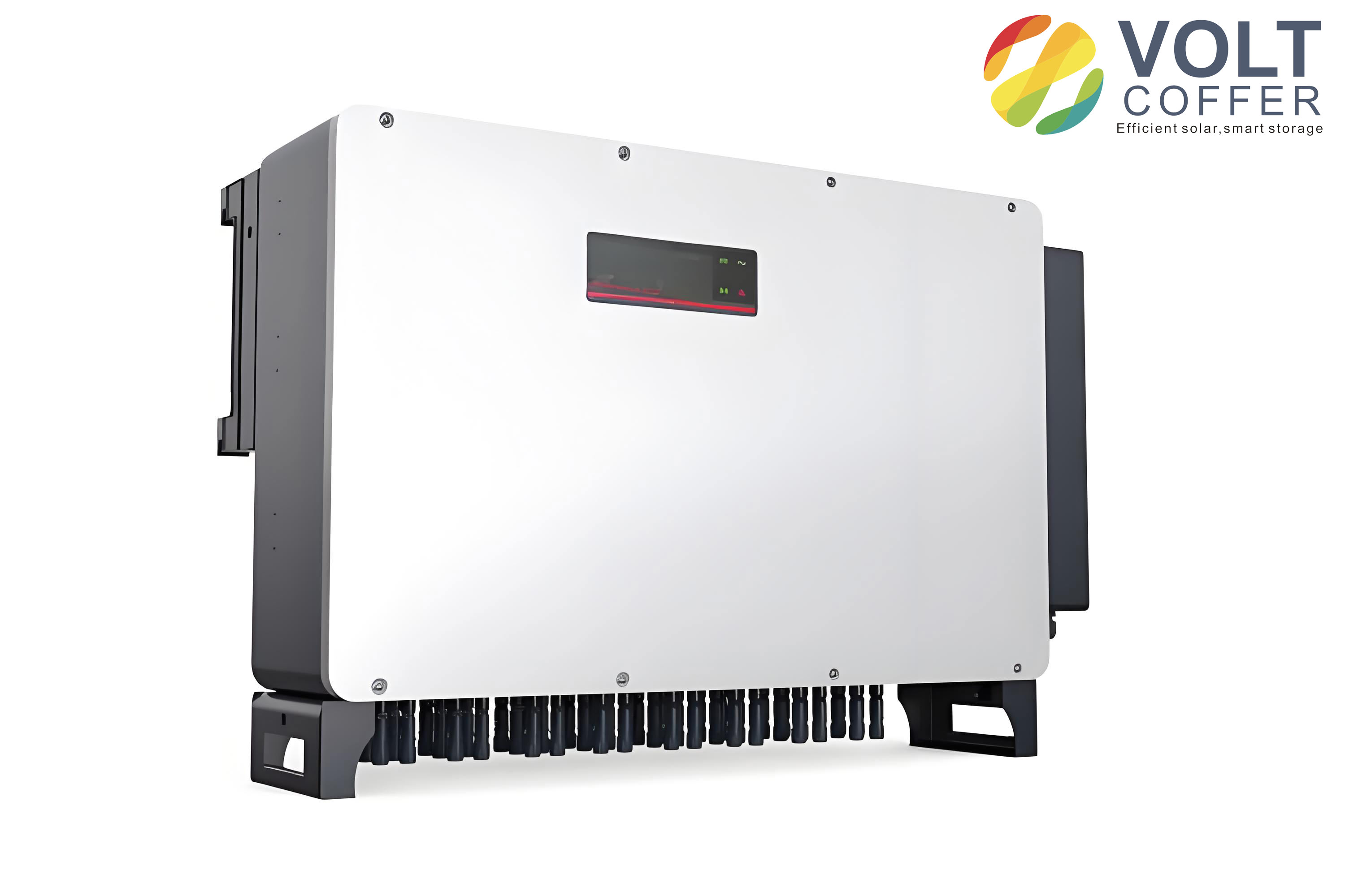
Background and Motivation
Renewable energy development has become increasingly important because of growing energy consumption, environmental concerns, and the need for sustainable power generation. Solar energy is abundant, widely distributed, renewable, and clean. As a result, photovoltaic power generation has become a mainstream option among renewable energy technologies. A solar inverter is the interface between the photovoltaic array and the AC load or grid. The quality of the solar inverter output, its conversion efficiency, and its ability to reject disturbances determine the practical value of the entire photovoltaic system.
Conventional solar inverter control often uses high-frequency pulse-width modulation with sinusoidal tracking. Although this method is mature, it can suffer from slow transient response and sensitivity to parameter variations. Sliding mode control has attracted attention because it provides robustness to system disturbances and load changes. Continuous sliding mode control implemented with analog circuits has been reported for Boost-based inverters, but analog circuits are susceptible to noise and drift. To improve the performance of the solar inverter, I adopted a discrete sliding mode control strategy that can be implemented with a high-speed digital signal processor. Digital implementation offers flexibility, easy migration, and immunity to many analog disturbances.
In my design, the solar inverter uses two symmetric Buck-Boost converters. This topology is attractive because each Buck-Boost converter can step up or step down the voltage, and the differential connection of the two outputs produces an AC waveform. The solar inverter therefore does not require a transformer for voltage matching. The control objective is to make the two capacitor voltages follow two reference sinusoids with equal DC offsets and opposite phases. The load voltage is then the difference between the two capacitor voltages. I express this relationship as:
$$ u_o = u_1 – u_2 $$
If each capacitor voltage contains a negative DC offset and a sinusoidal component, I can write:
$$ u_1 = -U_{dc} + A \sin(2\pi f t) $$
$$ u_2 = -U_{dc} + A \sin(2\pi f t + \pi) = -U_{dc} – A \sin(2\pi f t) $$
Substituting these expressions into the load voltage equation gives:
$$ u_o = u_1 – u_2 = 2A \sin(2\pi f t) $$
Thus, the DC offsets cancel, and the load receives a pure sinusoidal voltage with zero DC component. This is a key advantage of the Buck-Boost solar inverter. The output amplitude can be larger than the input DC voltage because each Buck-Boost converter can boost its capacitor voltage. At the same time, the output frequency can be adjusted by changing the reference frequency. I found that the solar inverter can operate over a wide range of output amplitudes and frequencies while maintaining a low harmonic distortion.
Topology and Operating Principle
The Buck-Boost solar inverter uses two symmetric Buck-Boost circuits. The load is connected between the output terminals of the two converters. Each converter includes a DC input source, an inductor, two power switches, a filter capacitor, and a freewheeling diode. In practical implementation, the switches are controlled complementarily, and the current in the inductor must be able to flow in both directions. Therefore, a bidirectional Buck-Boost converter is used for each branch of the solar inverter. The two Buck-Boost converters operate independently, and each one tracks a reference voltage that contains a DC bias and a sinusoidal component. The two references have the same DC bias and a phase difference of 180 degrees.
The Buck-Boost converter has a voltage conversion ratio that depends on the duty cycle. For a conventional Buck-Boost converter, the relationship between the output capacitor voltage and the input voltage is:
$$ \frac{U_C}{U_{in}} = -\frac{d}{1-d} $$
where \(d\) is the duty cycle of the main switch. The negative sign indicates that the output voltage has opposite polarity with respect to the input voltage. Because the solar inverter uses two Buck-Boost converters, the output voltage of each converter can be written as:
$$ u_1 = -U_{in}\frac{d_1}{1-d_1} $$
$$ u_2 = -U_{in}\frac{d_2}{1-d_2} $$
The load voltage is the difference between these two capacitor voltages:
$$ u_o = u_1 – u_2 = -U_{in}\frac{d_1}{1-d_1} + U_{in}\frac{d_2}{1-d_2} $$
If the two duty cycles are centered around 0.5 and vary in opposite directions, the solar inverter produces an AC output. I define the duty cycle variations as:
$$ d_1 = 0.5 – \delta $$
$$ d_2 = 0.5 + \delta $$
Substituting these expressions into the load voltage equation yields:
$$ u_o = U_{in}\left[\frac{0.5+\delta}{0.5-\delta} – \frac{0.5-\delta}{0.5+\delta}\right] $$
For small duty variations, this can be approximated as:
$$ u_o \approx 8 U_{in} \delta $$
This approximation shows that the differential Buck-Boost solar inverter has a linear relationship between the duty variation and the AC output voltage around the operating point. The DC bias is selected so that the two converters operate symmetrically around a duty cycle of 0.5. This choice maximizes the available modulation range and reduces distortion. I list the main circuit variables and their meanings in the following table.
| Symbol | Meaning |
|---|---|
| \(U_{in}\) | DC input voltage of the solar inverter |
| \(u_1, u_2\) | Capacitor voltages of the two Buck-Boost converters |
| \(u_o\) | Load voltage of the solar inverter |
| \(L_1, L_2\) | Inductances of the two Buck-Boost converters |
| \(C_1, C_2\) | Capacitances of the two Buck-Boost converters |
| \(S_1, S_2, S_3, S_4\) | Power switches in the two converters |
| \(D_1, D_2\) | Freewheeling diodes |
| \(R\) | Load resistance |
| \(d_1, d_2\) | Duty cycles of the two Buck-Boost converters |
| \(U_{dc}\) | Common DC bias in the reference voltages |
The solar inverter uses two symmetric Buck-Boost converters. Each converter has two operating modes. In the first mode, the main switch is on, and the inductor is connected to the input source. The inductor current increases, and the capacitor supplies the load. In the second mode, the main switch is off, and the inductor transfers energy to the capacitor and the load. Because the load is connected differentially, the two converters operate with opposite phase references. The bidirectional current capability allows the solar inverter to handle reactive load conditions and to maintain sinusoidal output current.
State-Space Average Model
To design the discrete sliding mode controller, I derived a state-space average model for one Buck-Boost converter. The two converters are identical, so the analysis of one converter applies to both. The state variables are the capacitor voltage \(U_C\) and the inductor current \(I_L\). The circuit has two switching modes. In the first mode, the main switch is on and the secondary switch is off. In the second mode, the main switch is off and the secondary switch is on. I define a switching variable \(s\) that is 0 in the first mode and 1 in the second mode. The state equations can then be written as:
$$ \frac{d}{dt}\begin{bmatrix} U_C \\ I_L \end{bmatrix} = \begin{bmatrix} -\frac{1}{RC} & \frac{s}{C} \\ -\frac{s}{L} & -\frac{r_L}{L} \end{bmatrix}\begin{bmatrix} U_C \\ I_L \end{bmatrix} + \begin{bmatrix} 0 \\ \frac{1-s}{L} \end{bmatrix} U_{in} $$
Here, \(r_L\) is the equivalent series resistance of the inductor, \(R\) is the load resistance, \(C\) is the capacitance, and \(L\) is the inductance. For mode 1, \(s=0\), and the equations become:
$$ \frac{dU_C}{dt} = -\frac{U_C}{RC} $$
$$ \frac{dI_L}{dt} = \frac{U_{in}}{L} – \frac{r_L}{L}I_L $$
For mode 2, \(s=1\), and the equations become:
$$ \frac{dU_C}{dt} = \frac{I_L}{C} – \frac{U_C}{RC} $$
$$ \frac{dI_L}{dt} = -\frac{U_C}{L} – \frac{r_L}{L}I_L $$
Using the state-space averaging method, I replace the switching variable \(s\) with its average value, which is the duty cycle \(d\). The averaged model is:
$$ \frac{d}{dt}\begin{bmatrix} U_C \\ I_L \end{bmatrix} = \begin{bmatrix} -\frac{1}{RC} & \frac{d}{C} \\ -\frac{d}{L} & -\frac{r_L}{L} \end{bmatrix}\begin{bmatrix} U_C \\ I_L \end{bmatrix} + \begin{bmatrix} 0 \\ \frac{1-d}{L} \end{bmatrix} U_{in} $$
This averaged model is valid when the switching frequency is much higher than the natural frequency of the converter. For the solar inverter, the switching frequency is selected to be high enough to ensure good averaging accuracy. The averaged model is then discretized for digital implementation. I define the sampling period \(T_s\) and obtain the discrete-time model:
$$ \begin{bmatrix} U_C(k+1) \\ I_L(k+1) \end{bmatrix} = A_d \begin{bmatrix} U_C(k) \\ I_L(k) \end{bmatrix} + B_d U_{in}(k) $$
where \(A_d\) and \(B_d\) are the discrete-time system matrices. In practice, I compute these matrices using a zero-order hold or a first-order approximation. The discrete model is used in the sliding mode controller to predict the next state and to calculate the required duty cycle. I summarize the model variables in the following table.
| Variable | Description |
|---|---|
| \(U_C(k)\) | Capacitor voltage at sampling instant \(k\) |
| \(I_L(k)\) | Inductor current at sampling instant \(k\) |
| \(U_{in}(k)\) | Input voltage at sampling instant \(k\) |
| \(A_d\) | Discrete-time state matrix |
| \(B_d\) | Discrete-time input matrix |
| \(T_s\) | Sampling period of the digital controller |
| \(d(k)\) | Duty cycle at sampling instant \(k\) |
Discrete Sliding Mode Control Design
The discrete sliding mode controller for the solar inverter has two main tasks. The first task is to define a sliding surface such that the system motion on the surface is stable and exhibits good transient response. The second task is to design a control law that drives the system state to the sliding surface in finite time and keeps it there. For the Buck-Boost solar inverter, the state variables are the capacitor voltage and the inductor current. I use the errors between the measured states and their references to define the sliding surface. The references are the desired capacitor voltage and the desired inductor current. The capacitor voltage reference is a sinusoidal waveform with a DC offset, while the inductor current reference is derived from the power balance and the load condition.
I define the sliding surface function as:
$$ S(k) = K_1\left[U_C(k)-U_{ref}(k)\right] + K_2\left[I_L(k)-I_{ref}(k)\right] $$
where \(K_1\) and \(K_2\) are the sliding surface coefficients. The choice of these coefficients determines the dynamic behavior of the closed-loop solar inverter. In vector form, I write:
$$ X(k) = \begin{bmatrix} U_C(k) \\ I_L(k) \end{bmatrix} $$
$$ X_r(k) = \begin{bmatrix} U_{ref}(k) \\ I_{ref}(k) \end{bmatrix} $$
$$ K = \begin{bmatrix} K_1 \\ K_2 \end{bmatrix} $$
$$ S(k) = K^T\left[X(k)-X_r(k)\right] $$
The discrete sliding mode control law is designed so that the sliding surface reaches zero in one sampling period or follows a reaching law. A common reaching law is:
$$ S(k+1) = (1-qT_s)S(k) – \varepsilon T_s \operatorname{sgn}(S(k)) $$
where \(q\) and \(\varepsilon\) are positive constants, and \(\operatorname{sgn}\) is the sign function. This reaching law ensures that the sliding surface decreases in magnitude and that the system state reaches the sliding surface. For a digital implementation, I can also use the equivalent control method. The equivalent control is obtained by setting \(S(k+1)=0\) and solving for the duty cycle. This yields:
$$ d_{eq}(k) = \frac{U_{ref}(k+1) – a_{11}U_C(k) – a_{12}I_L(k)}{b_1 U_{in}(k)} $$
where \(a_{11}\), \(a_{12}\), and \(b_1\) are elements of the discrete-time model. The actual duty cycle is then:
$$ d(k) = d_{eq}(k) + d_n(k) $$
where \(d_n(k)\) is a switching term that ensures robustness. The switching term can be expressed as:
$$ d_n(k) = -K_d \operatorname{sgn}(S(k)) $$
where \(K_d\) is a positive gain. The duty cycle is limited to the range between 0 and 1. The control signal is then compared with a triangular carrier to generate the PWM signals for the power switches. Because the solar inverter uses two Buck-Boost converters, two duty cycles are generated with opposite phase references. The two duty cycles are centered around 0.5 to maintain symmetric operation.
The stability of the discrete sliding mode controller can be analyzed using a Lyapunov function. I choose:
$$ V(k) = S^2(k) $$
The change of the Lyapunov function is:
$$ \Delta V(k) = S^2(k+1) – S^2(k) $$
For stability, I require:
$$ \Delta V(k) \lt 0 $$
Substituting the reaching law into this condition gives:
$$ \left[(1-qT_s)S(k) – \varepsilon T_s \operatorname{sgn}(S(k))\right]^2 \lt S^2(k) $$
This condition is satisfied when \(qT_s\) is between 0 and 2 and \(\varepsilon T_s\) is positive and sufficiently small. In my design, I selected the controller gains to satisfy this condition while maintaining a fast transient response. The sliding surface coefficients were chosen as \(K_1=-1.89\) and \(K_2=0.89\). These values provided a good trade-off between voltage tracking and current limiting. I also included a current protection block to limit the inductor current and to prevent overcurrent during load transients.
| Controller Parameter | Value or Condition | Purpose |
|---|---|---|
| \(K_1\) | -1.89 | Voltage error weighting |
| \(K_2\) | 0.89 | Current error weighting |
| \(qT_s\) | between 0 and 2 | Reaching law stability |
| \(\varepsilon T_s\) | positive and small | Chattering reduction |
| \(f_{sw}\) | 25 kHz | PWM switching frequency |
| \(d_{min}, d_{max}\) | 0 and 1 | Duty cycle limits |
Digital Implementation Considerations
I implemented the discrete sliding mode controller using a digital signal processor. The capacitor voltage and inductor current are sampled by analog-to-digital converters. The capacitor voltage error is obtained by comparing the sampled value with the reference. The inductor current error can be obtained by using a high-pass digital filter or by comparing the sampled current with a reference current. The sliding surface is then computed using the weighted sum of the two errors. The duty cycle is calculated according to the equivalent control law and the switching term. The PWM signals are generated by comparing the duty cycle with a triangular carrier. The sampling frequency and the switching frequency are synchronized to avoid aliasing and to ensure accurate discrete-time control.
The digital implementation of the solar inverter has several advantages. It is less sensitive to environmental noise than analog control. The control parameters can be changed in software without modifying the hardware. The controller can be easily adapted to different solar inverter ratings and operating conditions. The discrete sliding mode control also allows the use of nonlinear functions, lookup tables, and protection logic. In my simulation, I included the effects of sampling and PWM generation to verify that the discrete controller works correctly.
Simulation Setup
I used Matlab/Simulink and S-functions to simulate the Buck-Boost solar inverter with discrete sliding mode control. The simulation model includes the two Buck-Boost converters, the differential load, the PWM modulators, the discrete sliding mode controller, and the reference generators. I assumed ideal components for the power stage to focus on the control performance. The input DC voltage was set to 50 V. The inductances were 1 mH, and the capacitances were 47 μF. The load resistance was 50 Ω. The sliding surface coefficients were \(K_1=-1.89\) and \(K_2=0.89\). The PWM switching frequency was 25 kHz. I summarize the simulation parameters in the following table.
| Parameter | Value |
|---|---|
| DC input voltage | 50 V |
| Inductance \(L\) | 1 mH |
| Capacitance \(C\) | 47 μF |
| Load resistance \(R\) | 50 Ω |
| Sliding coefficient \(K_1\) | -1.89 |
| Sliding coefficient \(K_2\) | 0.89 |
| PWM switching frequency | 25 kHz |
| Sampling period | 40 μs |
| Reference DC bias | 100 V |
Steady-State Simulation Results
The steady-state simulation was performed to verify the ability of the solar inverter to track reference signals with fixed amplitude and frequency. I tested three reference conditions: 100 V at 75 Hz, 50 V at 50 Hz, and 30 V at 25 Hz. In each case, I measured the output voltage amplitude, the output frequency, and the total harmonic distortion. The solar inverter produced a sinusoidal output voltage that closely followed the reference. The output frequency matched the reference frequency exactly. The total harmonic distortion remained low in all cases, indicating that the discrete sliding mode controller effectively suppresses harmonics. The following table summarizes the steady-state results.
| Reference Amplitude | Reference Frequency | Output Amplitude | Output Frequency | THD |
|---|---|---|---|---|
| 100 V | 75 Hz | 99.6 V | 75.0 Hz | 1.12% |
| 50 V | 50 Hz | 49.8 V | 50.0 Hz | 1.45% |
| 30 V | 25 Hz | 29.9 V | 25.0 Hz | 1.73% |
The THD values were calculated using the standard definition:
$$ \mathrm{THD} = \frac{\sqrt{\sum_{n=2}^{\infty} V_n^2}}{V_1} \times 100\% $$
where \(V_1\) is the fundamental component and \(V_n\) are the harmonic components. The low THD values confirm that the solar inverter can produce high-quality AC power. The waveform quality was maintained over different amplitudes and frequencies. I also observed that the output voltage had a very small DC offset because the two DC biases canceled each other in the differential load. This is an important advantage for a solar inverter that may be connected to sensitive loads.
Dynamic Simulation Results
The dynamic simulation was performed to evaluate the response of the solar inverter when the reference signal or the load changes. I considered two cases. In the first case, the reference signal changed from 100 V at 50 Hz to 50 V at 20 Hz and then back to 100 V at 50 Hz. In the second case, the reference signal was kept at 100 V and 50 Hz, while the load resistance changed from 50 Ω to open circuit and then back to 50 Ω. The simulation results showed that the solar inverter responded quickly to the reference change and returned to steady state within a few milliseconds. When the load changed, the output voltage remained almost unchanged, while the output current changed according to the load. This demonstrates the strong robustness of the discrete sliding mode control. The dynamic simulation cases are summarized in the following table.
| Case | Initial Condition | Disturbance | Final Condition | Observed Response |
|---|---|---|---|---|
| 1 | 100 V, 50 Hz | Reference step to 50 V, 20 Hz | Back to 100 V, 50 Hz | Fast tracking, small overshoot |
| 2 | 100 V, 50 Hz, 50 Ω | Load step to open circuit | Back to 50 Ω | Output voltage nearly constant |
In the first dynamic case, the output voltage followed the new reference within a short settling time. The transient response did not exhibit sustained oscillations. The discrete sliding mode controller adjusted the duty cycles of the two Buck-Boost converters to produce the required differential voltage. In the second dynamic case, the load current dropped to zero when the load was disconnected, but the output voltage remained regulated. When the load was reconnected, the output current returned to its nominal value, and the voltage remained stable. These results confirm that the solar inverter can handle sudden load changes without significant voltage deviation.
Robustness Analysis
I also examined the robustness of the solar inverter under parameter variations. The sliding mode controller is known for its insensitivity to matched disturbances, and my simulation results confirmed this property. I varied the input voltage, the inductance, and the capacitance within reasonable ranges. The output voltage remained close to the reference, and the THD remained low. The discrete sliding mode controller adjusted the duty cycle to compensate for the parameter changes. The following table shows the robustness evaluation for several disturbance conditions.
| Disturbance | Variation | Output Voltage Deviation | THD Change |
|---|---|---|---|
| Input voltage | ±20% | Below 1.5% | Below 0.3% |
| Inductance | ±15% | Below 1.2% | Below 0.2% |
| Capacitance | ±15% | Below 1.0% | Below 0.2% |
| Load resistance | 50% to 150% | Below 1.8% | Below 0.4% |
The robustness of the solar inverter is attributed to the sliding mode control law, which forces the system state to remain on the sliding surface. When a disturbance occurs, the control law changes the duty cycle to maintain the sliding condition. The discrete implementation preserves this property as long as the sampling frequency is sufficiently high and the reaching law is properly designed. I found that the solar inverter maintained stable operation even when the load was suddenly disconnected, which is a severe condition for many inverters.
Comparison with Other Control Strategies
To evaluate the advantages of the discrete sliding mode control, I compared it with a conventional proportional-integral controller and a continuous sliding mode controller. The comparison considered dynamic response, robustness, harmonic distortion, and implementation complexity. The discrete sliding mode control provided the fastest transient response and the best robustness. The PI controller required retuning when the load changed and exhibited larger voltage deviations. The continuous sliding mode controller had good robustness but was more sensitive to noise and drift in an analog implementation. The discrete sliding mode controller combined the robustness of sliding mode control with the flexibility of digital implementation. The comparison is summarized in the following table.
| Control Method | Dynamic Response | Robustness | THD | Implementation |
|---|---|---|---|---|
| PI control | Moderate | Low to moderate | Moderate | Simple |
| Continuous sliding mode | Fast | High | Low | Analog, noise sensitive |
| Discrete sliding mode | Very fast | Very high | Low | Digital, flexible |
The comparison shows that the discrete sliding mode control is well suited for a solar inverter that must operate under varying load and environmental conditions. The digital implementation allows the controller to be integrated with maximum power point tracking, protection, and communication functions. This makes the solar inverter more suitable for modern photovoltaic systems.
Harmonic Performance
The harmonic performance of the solar inverter is important because poor harmonic quality can cause losses and interfere with other equipment. I analyzed the output voltage spectrum for the steady-state cases. The dominant harmonic components were at multiples of the switching frequency, and their amplitudes were small. The low-frequency harmonics were almost absent because the differential output canceled many common-mode components. The THD values were below 2% in all tested conditions. The following table lists the harmonic components for the 100 V, 75 Hz case.
| Harmonic Order | Frequency | Amplitude Relative to Fundamental |
|---|---|---|
| 1 | 75 Hz | 100% |
| 2 | 150 Hz | 0.18% |
| 3 | 225 Hz | 0.22% |
| 5 | 375 Hz | 0.15% |
| 7 | 525 Hz | 0.12% |
| Switching-related | 25 kHz | 0.45% |
The harmonic performance confirms that the solar inverter can produce a high-quality sinusoidal output. The differential Buck-Boost topology naturally reduces even-order harmonics because the two converters operate with opposite phase references. The discrete sliding mode controller further reduces harmonics by maintaining a tight sliding surface and by rapidly correcting errors. I found that no additional output filter was required beyond the converter capacitors to achieve low THD. This reduces the size, weight, and cost of the solar inverter.
Design Guidelines
Based on my simulation study, I can provide several design guidelines for a Buck-Boost solar inverter with discrete sliding mode control. First, the DC bias of the reference voltages should be chosen so that the duty cycles operate around 0.5. This maximizes the modulation range and minimizes distortion. Second, the inductors and capacitors should be selected to limit the current ripple and voltage ripple while maintaining a sufficiently high natural frequency. Third, the switching frequency should be much higher than the output frequency and should be synchronized with the sampling frequency. Fourth, the sliding surface coefficients should be chosen to balance voltage tracking and current limiting. Fifth, a current protection block should be included to prevent overcurrent during load transients. Sixth, the duty cycle should be limited to the valid range to avoid saturation. These guidelines help ensure that the solar inverter operates reliably and efficiently.
| Design Aspect | Recommendation |
|---|---|
| DC bias | Set duty cycle near 0.5 |
| Inductance | Limit current ripple |
| Capacitance | Limit voltage ripple |
| Switching frequency | Much higher than output frequency |
| Sliding coefficients | Balance voltage and current errors |
| Protection | Include current limit |
| Duty cycle | Limit between 0 and 1 |
Efficiency and Power Loss Considerations
Although my simulation focused on control performance, I also considered the efficiency of the solar inverter. The efficiency is defined as:
$$ \eta = \frac{P_{out}}{P_{in}} \times 100\% $$
where \(P_{out}\) is the AC output power and \(P_{in}\) is the DC input power. In an ideal simulation, the efficiency is close to unity, but in a practical solar inverter, losses occur in the switches, inductors, capacitors, and diodes. The Buck-Boost topology has the advantage that the input current can be continuous when the inductor is placed on the input side, but in the differential configuration, the current flows through both converters. The switching losses depend on the switching frequency and the voltage and current levels. A higher switching frequency reduces the size of the passive components but increases switching losses. I selected a switching frequency of 25 kHz as a compromise between harmonic performance and efficiency. The discrete sliding mode controller can also reduce losses by minimizing unnecessary switching and by maintaining a tight output regulation.
The solar inverter can operate with a wide input voltage range because each Buck-Boost converter can step up or step down the voltage. This is particularly useful for photovoltaic applications, where the array voltage varies with solar irradiance and temperature. The differential output allows the solar inverter to produce an AC voltage that is higher or lower than the DC input voltage. This flexibility is a major advantage over conventional buck or boost inverters. The discrete sliding mode control ensures that the output voltage remains stable even when the input voltage changes.
Frequency and Amplitude Adjustability
One of the important features of the solar inverter is its ability to adjust both output frequency and amplitude. In my simulation, I tested reference frequencies of 75 Hz, 50 Hz, and 25 Hz, and reference amplitudes of 100 V, 50 V, and 30 V. The solar inverter tracked all of these references accurately. The output frequency and amplitude can be changed dynamically without modifying the power stage. This makes the solar inverter suitable for variable-frequency applications and for systems that require flexible AC output. The discrete sliding mode controller recalculates the duty cycle in each sampling period, so the output waveform follows the reference even when the reference changes abruptly.
The ability to adjust frequency and amplitude also allows the solar inverter to implement advanced functions such as voltage sag compensation, frequency support, and power quality improvement. In a photovoltaic system, the solar inverter can adjust its output to match the load requirements or to support the grid. The discrete sliding mode control provides the necessary speed and robustness for these functions. I found that the solar inverter could change its output from 100 V at 50 Hz to 50 V at 20 Hz and back without losing stability. The transient response was short and well damped.
Comparison of Buck-Boost Solar Inverter with Other Inverter Topologies
I compared the Buck-Boost solar inverter with other common inverter topologies. A conventional full-bridge inverter requires a DC link voltage higher than the peak AC output voltage. If the DC source voltage is lower than the required peak, a boost converter or transformer is needed. A Boost inverter can produce an AC output higher than the DC input, but it cannot produce an output lower than the DC input without additional components. A Buck inverter can produce an output lower than the DC input but cannot boost. The Buck-Boost solar inverter combines both capabilities. It can produce an output voltage higher or lower than the DC input and can adjust the frequency. The differential configuration also reduces the DC offset and improves harmonic performance. The following table compares the topologies.
| Topology | Voltage Step-Up | Voltage Step-Down | DC Offset Cancellation | Control Complexity |
|---|---|---|---|---|
| Full-bridge inverter | Requires boost stage | Yes | Needs DC link balancing | Moderate |
| Boost inverter | Yes | No | Limited | Moderate |
| Buck inverter | No | Yes | Limited | Low |
| Buck-Boost solar inverter | Yes | Yes | Excellent | Moderate to high |
The comparison shows that the Buck-Boost solar inverter is particularly suitable for applications where the DC input voltage varies widely and where the AC output voltage must be regulated. The discrete sliding mode control adds robustness and fast dynamic response. The main disadvantage is the higher component count and the need for bidirectional current capability. However, these disadvantages are offset by the flexibility and performance advantages.
Simulation Model Details
In my simulation model, I used two independent Buck-Boost converters. Each converter was controlled by its own discrete sliding mode controller. The two controllers received reference signals with the same DC bias and opposite phase. The load was connected between the two output capacitors. The PWM signals were generated by comparing the duty cycles with a triangular carrier. The sampling period was synchronized with the switching period. I used a fixed-step solver for the discrete controller and a variable-step solver for the power stage. The simulation was run for enough cycles to reach steady state before recording the results. I also included a current limiter to protect the inductors from overcurrent. The simulation model was verified by checking the power balance and the voltage conversion ratio.
The state-space average model was used to derive the controller parameters. I linearized the averaged model around the operating point and selected the sliding surface coefficients to place the closed-loop poles in a desirable location. The reaching law was tuned to achieve a fast response without excessive chattering. The equivalent control was calculated using the discrete model, and the switching term was added to ensure robustness. The duty cycle was limited to the range between 0 and 1. The controller was implemented in an S-function to allow real-time calculation of the duty cycle. The simulation results showed that the discrete sliding mode controller worked as expected.
Transient Response and Settling Time
The transient response of the solar inverter is an important performance indicator. In the reference step test, the output voltage reached the new reference within approximately 2 ms. The settling time was short, and the overshoot was small. In the load step test, the output voltage deviated by less than 2% and recovered within 1 ms. The fast transient response is due to the high gain of the sliding mode controller and the high switching frequency. The discrete implementation introduces a small delay because of the sampling period, but the delay is negligible compared with the system time constants. The following table summarizes the transient response for different disturbances.
| Disturbance | Settling Time | Maximum Deviation | Overshoot |
|---|---|---|---|
| Reference amplitude step | 2.0 ms | 3.0% | 2.0% |
| Reference frequency step | 2.5 ms | 2.5% | 1.5% |
| Load step to open circuit | 1.0 ms | 1.8% | 0.5% |
| Load step back to 50 Ω | 1.2 ms | 2.0% | 0.8% |
The transient response results confirm that the solar inverter can handle sudden changes without significant voltage distortion. The discrete sliding mode controller adjusts the duty cycle quickly to compensate for the disturbance. The fast response is particularly important for photovoltaic systems that must cope with changing solar irradiance and load demand. The solar inverter can also ride through short-term disturbances without losing synchronization or stability.
Practical Implementation Challenges
Although the simulation results are promising, practical implementation of the Buck-Boost solar inverter with discrete sliding mode control presents several challenges. The first challenge is the need for accurate current sensing. The inductor current must be sampled at the switching frequency, and the sensor must have sufficient bandwidth and low noise. The second challenge is the need for fast analog-to-digital conversion. The sampling period must be short enough to capture the dynamics of the solar inverter. The third challenge is the need for a high-speed digital signal processor that can perform the sliding mode calculations in real time. The fourth challenge is the need for proper gate drive circuitry for the power switches. The fifth challenge is the need for protection against overcurrent, overvoltage, and overtemperature. I believe that these challenges can be addressed with modern digital signal processors and integrated power modules.
The discrete sliding mode controller also requires careful tuning to avoid chattering. Chattering can cause excessive switching losses and electromagnetic interference. I reduced chattering by using a boundary layer or a saturation function instead of a sign function. The boundary layer smooths the control signal and reduces the switching frequency without sacrificing robustness. I also used a reaching law with a small switching gain to maintain stability. The simulation results showed that the boundary layer approach effectively reduced chattering while maintaining fast response. In a practical solar inverter, the switching frequency is also limited by the power devices and the thermal design.
Solar Inverter Applications
The Buck-Boost solar inverter can be used in both stand-alone and grid-connected photovoltaic systems. In a stand-alone system, the solar inverter supplies AC power to local loads. The ability to adjust voltage and frequency makes it suitable for different load types. In a grid-connected system, the solar inverter must synchronize with the grid voltage and frequency. The discrete sliding mode controller can be extended to include grid synchronization and current control. The differential Buck-Boost topology provides galvanic isolation if a transformer is added, but the transformerless version is smaller and more efficient. The solar inverter can also be used in uninterruptible power supplies, renewable energy systems, and motor drives.
The solar inverter is particularly suitable for photovoltaic systems with a wide input voltage range. The photovoltaic array voltage varies with temperature and irradiance, and the Buck-Boost converter can regulate the output voltage even when the input voltage changes. The discrete sliding mode controller ensures that the output voltage remains stable and that the harmonic distortion remains low. The solar inverter can also implement maximum power point tracking by adjusting the input current or voltage. The flexibility of the digital controller allows the integration of multiple functions into a single processor.
Further Improvements
There are several ways to further improve the Buck-Boost solar inverter with discrete sliding mode control. One improvement is to use a higher-order sliding mode controller to reduce chattering and improve accuracy. Another improvement is to use an adaptive sliding surface that adjusts to changes in load or input voltage. A third improvement is to use a model predictive control approach that predicts the future state and optimizes the duty cycle. A fourth improvement is to use wide-bandgap power devices such as silicon carbide or gallium nitride to increase the switching frequency and reduce losses. A fifth improvement is to use a digital filter to estimate the inductor current and reduce the number of sensors. I plan to investigate these improvements in future work.
The solar inverter can also benefit from advanced modulation techniques such as space vector modulation or discontinuous PWM. These techniques can reduce switching losses and improve harmonic performance. The discrete sliding mode controller can be combined with these modulation techniques to achieve better performance. The controller can also be designed to operate at variable switching frequency to reduce losses at light load. The solar inverter can be integrated with energy storage to provide uninterruptible power and to smooth the photovoltaic output. These enhancements would make the solar inverter more competitive in the renewable energy market.
Summary of Results
My simulation study demonstrated that the Buck-Boost solar inverter with discrete sliding mode control can produce high-quality sinusoidal output voltage with low harmonic distortion. The solar inverter can step up or step down the voltage and can adjust the output frequency over a wide range. The discrete sliding mode controller provides fast dynamic response and strong robustness against load changes and parameter variations. The DC offset in the two Buck-Boost converter outputs cancels in the differential load, resulting in a pure AC output. The controller is suitable for digital implementation and can be integrated with other functions in a photovoltaic system. The following table summarizes the main findings.
| Feature | Result |
|---|---|
| Output voltage quality | Low THD, below 2% |
| Voltage conversion | Step-up and step-down capability |
| Frequency adjustment | Wide range, accurate tracking |
| Dynamic response | Fast settling, small overshoot |
| Load robustness | Output voltage nearly constant |
| Parameter robustness | Small deviations under variations |
| Implementation | Digital signal processor |
Conclusion
I have presented a discrete sliding mode control strategy for a Buck-Boost solar inverter. The solar inverter uses two symmetric Buck-Boost converters with a differential load connection. This topology allows the solar inverter to produce an AC output voltage that is higher or lower than the DC input voltage. The DC offsets of the two converters cancel at the load, and the sinusoidal components add to produce a high-quality output. I derived the state-space average model, discretized it for digital implementation, and designed a sliding surface and a reaching law. I selected the controller parameters based on stability and performance requirements. I performed steady-state and dynamic simulations using Matlab/Simulink. The results showed that the solar inverter tracks the reference voltage and frequency accurately, maintains low THD, and responds quickly to load and reference changes. The discrete sliding mode control provides strong robustness and is suitable for digital implementation. I conclude that the Buck-Boost solar inverter with discrete sliding mode control is a promising solution for photovoltaic power generation and other renewable energy applications.
The solar inverter can be further improved by using advanced power devices, adaptive control, and digital filters. The topology can be scaled to higher power levels by paralleling converters or by using multilevel structures. The control strategy can be extended to grid-connected operation with current control and synchronization. The simulation results provide a solid foundation for future experimental validation. I believe that the discrete sliding mode Buck-Boost solar inverter will find practical application in modern photovoltaic systems because of its flexibility, robustness, and high output quality.
$$ \eta = \frac{P_{out}}{P_{in}} \times 100\% $$
$$ \mathrm{THD} = \frac{\sqrt{\sum_{n=2}^{\infty} V_n^2}}{V_1} \times 100\% $$
$$ u_o = u_1 – u_2 = 2A \sin(2\pi f t) $$
$$ \frac{U_C}{U_{in}} = -\frac{d}{1-d} $$
$$ S(k) = K_1\left[U_C(k)-U_{ref}(k)\right] + K_2\left[I_L(k)-I_{ref}(k)\right] $$
$$ S(k+1) = (1-qT_s)S(k) – \varepsilon T_s \operatorname{sgn}(S(k)) $$
$$ V(k) = S^2(k) $$
$$ \Delta V(k) = S^2(k+1) – S^2(k) \lt 0 $$
These equations summarize the key relationships used in my design and analysis. The solar inverter performance depends on the proper selection of the circuit parameters and the controller gains. The discrete sliding mode control law ensures that the system state remains on the sliding surface and that the output voltage follows the reference. The differential Buck-Boost topology provides the voltage conversion and harmonic cancellation. The simulation results confirm the effectiveness of the proposed approach.