
In the context of integrating distributed renewable energy sources into the main power network, the grid connected inverter serves as a critical interface. Its control performance directly impacts grid stability and power quality. Traditional control strategies, such as the dual-loop proportional-integral (PI) control, often exhibit limitations in dynamic response and robustness under varying grid conditions and reference changes. This work addresses these challenges by proposing a novel composite control strategy that synergizes differential flatness theory with quasi-proportional resonant (QPR) control. The primary objective is to achieve superior dynamic tracking, enhanced disturbance rejection, and improved grid current quality for single-phase grid connected inverters.
The proposed methodology leverages the inherent advantages of both frameworks. Differential flatness provides a systematic way to design trajectory-tracking controllers based on a system’s flat outputs, offering excellent dynamic performance and robustness without requiring an exact nonlinear model. Meanwhile, the quasi-proportional resonant controller is employed within the error feedback loop to ensure precise sinusoidal reference tracking and effective suppression of specific harmonics at the fundamental frequency, thereby elevating the quality of the injected grid current. This article presents a comprehensive derivation of the system model, controller design, and simulation-based validation, demonstrating the efficacy of the proposed Differential Flatness-QPR (DF-QPR) control strategy for single-phase grid connected inverters.
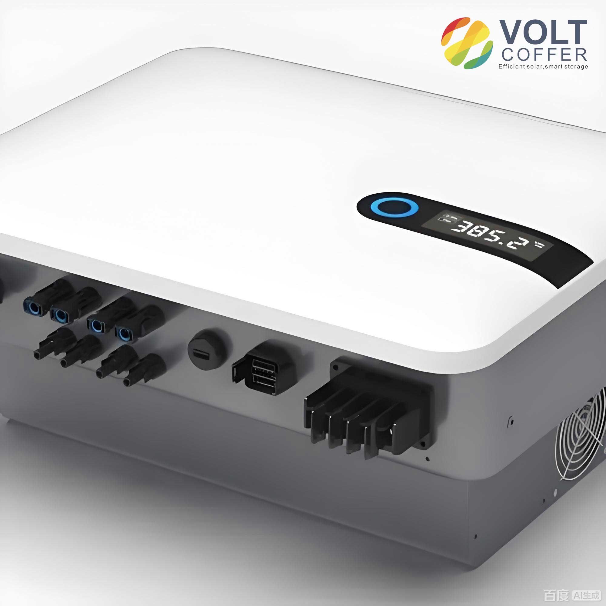
The foundational element of any control design is an accurate mathematical model. The topology under consideration is a single-phase full-bridge voltage source inverter with an LC output filter, a standard configuration for grid connected inverter applications. The key electrical parameters and variables are defined in the following table:
| Symbol | Description |
|---|---|
| $$U_{dc}$$ | DC-link voltage |
| $$L$$ | Filter inductance |
| $$C$$ | Filter capacitance |
| $$i_L$$ | Inductor current |
| $$v_C$$ | Capacitor voltage |
| $$v_g$$, $$i_g$$ | Grid voltage and current |
| $$v_{ab}$$ | Inverter bridge output voltage |
The dynamic equations in the stationary ($$\alpha\beta$$) frame are derived from Kirchhoff’s laws:
$$ L \frac{di_L}{dt} = v_{ab} – v_C $$
$$ C \frac{dv_C}{dt} = i_L – i_g $$
$$ v_g = v_C $$
For control design in a synchronous rotating (dq) frame, which simplifies the control of active and reactive power, a virtual orthogonal system must be constructed for the single-phase quantities. This is efficiently accomplished using a Second-Order Generalized Integrator (SOGI). The SOGI generates two orthogonal signals ($$\alpha$$ and $$\beta$$) from a single-phase input. Its transfer functions for an input signal $$x$$ and angular frequency $$\omega_0$$ are:
$$ H_{\alpha}(s) = \frac{x_{\alpha}(s)}{x(s)} = \frac{k \omega_0 s}{s^2 + k \omega_0 s + \omega_0^2} $$
$$ H_{\beta}(s) = \frac{x_{\beta}(s)}{x(s)} = \frac{k \omega_0^2}{s^2 + k \omega_0 s + \omega_0^2} $$
where $$k$$ is a damping factor typically set to $$\sqrt{2}$$ for optimal performance. Applying the SOGI to the grid voltage and current signals allows us to define the dq transformation. Aligning the d-axis with the grid voltage vector ($$V_{gd} = V_m, V_{gq}=0$$), the state-space model in the synchronous dq frame is obtained:
$$ L \frac{di_{Ld}}{dt} = v_{abd} – v_{Cd} – \omega_0 L i_{Lq} $$
$$ L \frac{di_{Lq}}{dt} = v_{abq} – v_{Cq} + \omega_0 L i_{Ld} $$
$$ C \frac{dv_{Cd}}{dt} = i_{Ld} – i_{gd} – \omega_0 C v_{Cq} $$
$$ C \frac{dv_{Cq}}{dt} = i_{Lq} – i_{gq} + \omega_0 C v_{Cd} $$
Here, the subscript ‘d’ and ‘q’ denote the direct and quadrature components, respectively, and $$\omega_0$$ is the grid angular frequency. The instantaneous active and reactive power delivered to the grid by the grid connected inverter are given by:
$$ P = \frac{1}{2} (v_{gd} i_{gd} + v_{gq} i_{gq}) = \frac{1}{2} V_m i_{gd} $$
$$ Q = \frac{1}{2} (v_{gq} i_{gd} – v_{gd} i_{gq}) = -\frac{1}{2} V_m i_{gq} $$
This model forms the basis for the subsequent differential flatness analysis and controller synthesis. The performance of the grid connected inverter hinges critically on the chosen control strategy.
Differential flatness is a powerful concept for the control of nonlinear systems. A system is considered differentially flat if one can find a set of outputs, called flat outputs, such that all system states and inputs can be expressed as algebraic functions of these flat outputs and a finite number of their time derivatives. This property allows for straightforward trajectory planning and feedforward control design. For our single-phase grid connected inverter system, we select the inductor current components as candidate flat outputs:
$$ \mathbf{y} = [y_1, y_2]^T = [i_{Ld}, i_{Lq}]^T $$
The state vector is chosen as $$\mathbf{x} = [i_{Ld}, i_{Lq}]^T$$ and the control input vector as $$\mathbf{u} = [v_{abd}, v_{abq}]^T$$. It is immediately evident that the states are trivially expressed by the flat outputs:
$$ \mathbf{x} = \boldsymbol{\varphi}(\mathbf{y}) = [y_1, y_2]^T $$
To express the inputs, we differentiate the flat outputs and substitute from the system model. From the dq-frame inductor equations, we can solve for the inputs:
$$ v_{abd} = L \dot{y}_1 + V_m + \omega_0 L y_2 $$
$$ v_{abq} = L \dot{y}_2 + \omega_0 L y_1 $$
where we used $$v_{Cd} \approx V_m$$ and $$v_{Cq} \approx 0$$, assuming a well-regulated capacitor voltage at the fundamental frequency. The expressions confirm that the inputs $$\mathbf{u}$$ can be written as functions of the flat outputs $$\mathbf{y}$$ and their first derivatives $$\dot{\mathbf{y}}$$. Therefore, the single-phase LC-type grid connected inverter is a differentially flat system. This property is exploited to design a controller with inherent feedforward action for excellent reference tracking.
The overall control structure for the grid connected inverter employs a cascade architecture: an outer power loop and an inner current loop. The outer loop computes the current references based on the desired active and reactive power. The inner loop regulates the inductor currents to these references. The novelty lies in applying differential flatness theory to both loops and enhancing the inner loop’s error feedback with a QPR controller.
Outer Power Loop (Differential Flatness Controller): The flat outputs for the power loop are the active and reactive power $$(P, Q)$$. However, from the power equations, the references for the dq currents serve as the immediate commands for the inner loop. Using the flatness principle, the feedforward terms for the current references are derived directly from the desired power trajectories $$P^*, Q^*$$:
$$ i_{Ld,ff}^* = \frac{2P^*}{V_m}, \quad i_{Lq,ff}^* = -\frac{2Q^*}{V_m} $$
To compensate for model inaccuracies and disturbances, a feedback correction is added. Defining power errors $$\Delta P = P^* – P$$ and $$\Delta Q = Q^* – Q$$, the feedback terms are generated via simple proportional-integral (PI) regulators:
$$ i_{Ld,fb}^* = \left( K_{p,P} + \frac{K_{i,P}}{s} \right) \Delta P $$
$$ i_{Lq,fb}^* = \left( K_{p,Q} + \frac{K_{i,Q}}{s} \right) \Delta Q $$
The final current references for the inner loop are the sum of feedforward and feedback components:
$$ i_{Ld}^* = i_{Ld,ff}^* + i_{Ld,fb}^*, \quad i_{Lq}^* = i_{Lq,ff}^* + i_{Lq,fb}^* $$
Inner Current Loop (Differential Flatness with QPR Feedback): The inner loop controls the actual inductor currents $$(i_{Ld}, i_{Lq})$$ to track the references $$(i_{Ld}^*, i_{Lq}^*)$$. Applying differential flatness again, the feedforward control voltages are computed from the reference currents and their derivatives:
$$ v_{abd,ff}^* = L \frac{di_{Ld}^*}{dt} + V_m + \omega_0 L i_{Lq}^* $$
$$ v_{abq,ff}^* = L \frac{di_{Lq}^*}{dt} + \omega_0 L i_{Ld}^* $$
These feedforward terms account for the system dynamics and provide the primary control effort for perfect tracking if the model is exact. The error feedback loop is responsible for rejecting disturbances, parameter variations, and compensating for any discrepancy between the model and the real grid connected inverter. Traditionally, PI controllers are used here. However, to achieve zero steady-state error for sinusoidal signals at the fundamental frequency and improve harmonic rejection, we propose using a Quasi-Proportional Resonant (QPR) controller. The transfer function of a QPR controller is:
$$ G_{QPR}(s) = K_p + \frac{2K_r \omega_c s}{s^2 + 2\omega_c s + \omega_0^2} $$
where $$K_p$$ is the proportional gain, $$K_r$$ is the resonant gain, $$\omega_0$$ is the resonant frequency (grid frequency), and $$\omega_c$$ is the cutoff frequency that determines the bandwidth of the resonant peak. This controller provides very high gain at $$\omega_0$$, forcing the error at that frequency to zero. The feedback control voltages are thus:
$$ v_{abd,fb}^* = G_{QPR}(s) (i_{Ld}^* – i_{Ld}) + \omega_0 L (i_{Lq}^* – i_{Lq}) $$
$$ v_{abq,fb}^* = G_{QPR}(s) (i_{Lq}^* – i_{Lq}) – \omega_0 L (i_{Ld}^* – i_{Ld}) $$
The cross-coupling terms $$\omega_0 L (i_{Lq}^* – i_{Lq})$$ and $$-\omega_0 L (i_{Ld}^* – i_{Ld})$$ are added for decoupling, improving the independent control of d and q axes. The final modulation signals sent to the PWM generator are:
$$ v_{abd}^* = v_{abd,ff}^* + v_{abd,fb}^*, \quad v_{abq}^* = v_{abq,ff}^* + v_{abq,fb}^* $$
This composite structure ensures that the grid connected inverter rapidly follows power commands while maintaining high-quality, low-harmonic grid currents. The following table summarizes the key controller parameters used in the simulation study:
| Controller | Parameter | Value | Role |
|---|---|---|---|
| Power Loop (PI) | $$K_{p,P}, K_{p,Q}$$ | 0.05 | Proportional gain |
| $$K_{i,P}, K_{i,Q}$$ | 2.0 | Integral gain | |
| Current Loop (QPR) | $$K_p$$ | 1.0 | Proportional gain |
| $$K_r$$ | 100 | Resonant gain | |
| $$\omega_c$$ | 5 rad/s | Cutoff frequency |
To validate the proposed DF-QPR control strategy, a detailed simulation model of the single-phase grid connected inverter is developed in MATLAB/Simulink. The system parameters are listed below. The performance is compared against a conventional dual-loop PI controller, where both the outer power loop and inner current loop use standard PI regulators.
| System Parameter | Symbol | Value |
|---|---|---|
| Grid Voltage (RMS) | $$V_g$$ | 220 V |
| Grid Frequency | $$f_0$$ | 50 Hz |
| DC-Link Voltage | $$U_{dc}$$ | 400 V |
| Filter Inductance | $$L$$ | 3 mH |
| Filter Capacitance | $$C$$ | 10 µF |
| Switching Frequency | $$f_{sw}$$ | 10 kHz |
Scenario 1: Step Change in Active Power Reference. Initially, the grid connected inverter is set to inject 1 kW of active power and 0 Var reactive power. At time t = 0.2 s, the active power reference steps to 2 kW. The dynamic response of active power, reactive power, and grid current is analyzed.
The simulation results clearly demonstrate the superiority of the DF-QPR controller. The active power response under DF-QPR control exhibits a significantly faster settling time and lower overshoot compared to the traditional PI control. The DF-QPR controller leverages its feedforward action to anticipate the change, resulting in near-instantaneous tracking. The conventional PI controller shows a sluggish response with noticeable oscillation. This directly translates to a more stable and responsive grid connected inverter. The reactive power, which should remain at zero, shows a much smaller and shorter-duration deviation for the DF-QPR controlled system, indicating better decoupling control.
Most importantly, the quality of the grid current is markedly improved. The grid current waveform under DF-QPR control is smooth and sinusoidal even during the transient. A Fast Fourier Transform (FFT) analysis reveals a total harmonic distortion (THD) of 1.8% for the DF-QPR controller, whereas the PI controller yields a THD of 4.5%. The high gain of the QPR controller at the fundamental frequency effectively suppresses tracking errors and associated low-order harmonics. The following table quantifies the performance metrics for this test:
| Metric | DF-QPR Control | PI Control |
|---|---|---|
| Settling Time (Power) | ~15 ms | ~50 ms |
| Overshoot (Power) | < 5% | > 20% |
| Grid Current THD | 1.8% | 4.5% |
Scenario 2: Grid Voltage Sag. To evaluate robustness, a 30% voltage sag is applied to the grid at t = 0.3 s, lasting for 0.1 s, while the power references remain constant. This is a critical test for any grid connected inverter control scheme, as it must maintain stability and proper current injection during grid faults.
The DF-QPR controlled system demonstrates excellent robustness. The active power shows a brief dip but recovers quickly to its reference value with minimal oscillation. The current remains sinusoidal and within safe limits. The traditional PI controller, in contrast, exhibits larger power fluctuations and a more distorted current waveform during the sag. The inherent decoupling and the precise tracking of the QPR controller help the DF-QPR strategy to better reject this grid-side disturbance. The ability to maintain high performance under such conditions is essential for the reliable operation of grid connected inverters in weak or unstable grids.
The mathematical analysis of the disturbance rejection can be linked to the sensitivity function. With the QPR controller in the loop, the sensitivity $$S(s)$$ at the resonant frequency $$\omega_0$$ is very small, meaning the system is less sensitive to disturbances or reference variations at that frequency. This is a key advantage for a grid connected inverter that must operate synchronously with the grid voltage.
$$ S(s) = \frac{1}{1 + G_{QPR}(s)G_p(s)} $$
where $$G_p(s)$$ is the plant transfer function from voltage to current. At $$s = j\omega_0$$, $$G_{QPR}(j\omega_0)$$ has a very large magnitude, driving $$S(j\omega_0)$$ close to zero.
In conclusion, this article has presented and validated a novel differential flatness-based quasi-proportional resonant control strategy for single-phase grid connected inverters. The proposed DF-QPR controller successfully addresses the common limitations of traditional PI control, namely, slow dynamic response, poor disturbance rejection, and higher grid current harmonic content. By combining the trajectory-planning strength of differential flatness feedforward with the precise sinusoidal tracking capability of the QPR feedback controller, the system achieves:
- Superior Dynamic Performance: Rapid and smooth tracking of step changes in power reference with minimal overshoot.
- Enhanced Robustness: Effective mitigation of performance degradation during grid voltage disturbances like sags.
- Improved Power Quality: Significant reduction in grid current total harmonic distortion (THD), leading to cleaner power injection.
The simulation studies under various operational scenarios confirm these advantages. The DF-QPR control strategy offers a compelling solution for enhancing the performance and reliability of single-phase grid connected inverters, which are pivotal in modern distributed energy systems. Future work may involve experimental validation on a hardware prototype, extension to three-phase systems, and adaptation for grid connected inverters operating under highly unbalanced or distorted grid conditions. Furthermore, the integration of adaptive mechanisms to tune the QPR parameters online could be explored to maintain optimal performance as grid impedance varies, making the grid connected inverter even more versatile and robust.