
In the rapidly expanding field of photovoltaic (PV) power generation, the testing and validation of grid-connected control systems, particularly the Automatic Generation Control (AGC) and Automatic Voltage Control (AVC) for PV plants, present significant challenges. As an engineer involved in the development of such systems, I have observed that traditional testing methods are inadequate. Independent laboratory tests often fail to replicate the large-scale, dynamic environments of actual PV plants, while on-site testing can lead to substantial energy losses and economic drawbacks for plant operators. These limitations hinder the functional upgrades and performance verification of PV AGC/AVC systems. To address these issues, our team has conceived and developed a virtual solar inverter model. This virtual entity mimics the behavior of physical solar inverters, enabling comprehensive testing without the need for a full-scale physical setup. In this article, I will elaborate on the design, implementation, and testing of this virtual solar inverter, emphasizing its role in facilitating robust PV AGC/AVC system validation.
The core objective is to create a software-based model that accurately simulates the operational characteristics of solar inverters. Solar inverters are critical components in PV plants, converting direct current (DC) from solar panels into alternating current (AC) for grid injection. They are also the primary devices regulated by PV AGC (for active power control) and PV AVC (for reactive power and voltage control). Our virtual solar inverter must replicate key functionalities: dynamic active power output influenced by weather variations, response to direct control commands (both active and reactive power setpoints), and simulation of various operational scenarios such as communication failures. By deploying multiple instances of this virtual model, we can construct a virtual PV plant of any desired capacity, thereby providing a scalable testbed for control system algorithms.
The architecture of our virtual solar inverter model is structured around several interdependent modules, as illustrated conceptually below. It integrates environmental inputs, control logic, and real-time calculation algorithms to determine output values.
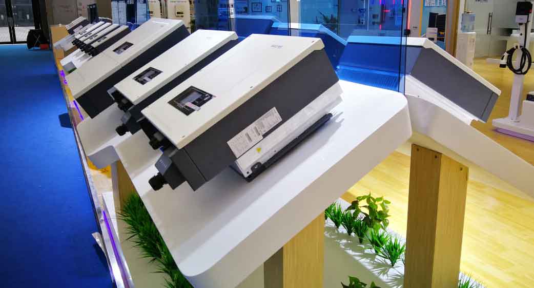
The design encompasses three primary aspects: model design, operational condition simulation, and mathematical formulation for output calculations.
Model Design and Functional Specifications
Our virtual solar inverter model is a simplified yet accurate representation of a physical solar inverter, focusing on attributes relevant to AGC/AVC testing. The model’s behavior is governed by three main factors: environmental (weather) conditions, external control inputs, and inherent inverter properties.
Weather Influence on Active Power
In real-world operation, the active power output of solar inverters fluctuates with solar irradiance, which is affected by weather conditions such as cloud cover, time of day, and season. To simulate this, our model incorporates a weather parameter text file. This file contains time-stamped records of active power values from an uncontrolled, freely generating inverter over a typical day. The data reflects the natural bell-shaped curve: power rising from morning to noon and declining towards evening. The model reads this file and dynamically adjusts the base active power output (\(P_{weather}\)) accordingly. This allows us to test the PV AGC system’s ability to track setpoints amidst natural power variability. The temporal resolution of the data can be configured (e.g., 1, 5, or 10-minute intervals) to simulate different granularities of weather-induced fluctuations.
Control Input Response
Solar inverters receive control commands, typically via tele-regulation (setpoint adjustment) or tele-control (on/off switching), from higher-level systems like the PV AGC/AVC. Our virtual model must accurately respond to such commands. The key control inputs are:
- Active Power Setpoint (\(P_{control}\)): Sent by the AGC application.
- Reactive Power Setpoint (\(Q_{control}\)): Sent by the AVC application.
- Breaker Status Command: A tele-control command for grid connection/disconnection.
Upon receiving a setpoint, the model updates its internal state and, after a configurable delay to simulate real-world response time, adjusts its output measurements. This simulates the closed-loop control process where the AGC/AVC issues commands and observes the resultant changes in inverter telemetry.
Inverter-Inherent Factors and Simplifications
While physical solar inverters from different manufacturers exhibit variations in efficiency, response time, and control characteristics, our initial model assumes homogeneity for simplicity. All virtual solar inverters in a test setup have identical performance parameters. This simplification is acceptable for system-level functional testing of the AGC/AVC logic. However, the model is designed to be extensible, allowing for the introduction of parameter variances to simulate a heterogeneous inverter fleet in future enhancements.
| Parameter | Symbol | Typical Range/Value | Description |
|---|---|---|---|
| Base Active Power (Weather) | \(P_{weather}\) | 0 to \(P_{max}\) kW | Derived from weather parameter file, represents maximum possible output under given irradiance. |
| Active Power Setpoint | \(P_{control}\) | 0 to \(P_{max}\) kW | Commanded value from AGC. |
| Active Power Limit | \(P_{limit}\) | 0 to \(P_{max}\) kW | Current operational limit imposed by AGC (e.g., due to grid constraints). |
| Reactive Power Setpoint | \(Q_{control}\) | \(-Q_{max}\) to \(+Q_{max}\) kvar | Commanded value from AVC. |
| Reactive Power Limit | \(Q_{limit}\) | \(-Q_{max}\) to \(+Q_{max}\) kvar | Current operational limit imposed by AVC. |
| Maximum Apparent Power | \(S_{max}\) | e.g., 550 kVA | Defines the inverter’s capacity constraint: \(P^2 + Q^2 \leq S_{max}^2\). |
| Response Delay | \(\tau\) | Configurable (e.g., 5-60 seconds) | Time between receiving a setpoint and achieving the output change. |
Simulation of Operational Conditions and Fault Scenarios
A robust test environment must account for non-ideal operating conditions. Our virtual solar inverter model includes simulations for communication failures and variable response times.
Communication Status Simulation
Communication links between inverters and the supervisory control system can fail. We model two distinct failure modes:
- Communication Interruption with Grid Connection: The inverter remains connected to the grid and generating power, but its data (telemetry) is not transmitted to the controller. In this case, the virtual solar inverter continues to compute its output based on weather and last received setpoint, but these values are not reported. The actual plant-level power is affected, but the controller is unaware of the individual inverter’s state.
- Communication Interruption due to Inverter Fault: The inverter has tripped offline (e.g., due to an internal fault). Here, its output is zero, and communication is lost. This represents a more severe condition where the inverter contributes nothing to the plant output.
The test operator can manually trigger these conditions at specified times to evaluate the AGC/AVC system’s resilience and fault-handling logic.
Response Time Variability
Physical solar inverters have finite and sometimes variable response times to control commands. Our model incorporates a configurable delay parameter (\(\tau\)). When a new setpoint is received, the model’s output does not change instantaneously. Instead, it transitions from the current value to the target value over a period defined by \(\tau\). This can be modeled as a first-order lag:
$$ P_{actual}(t) = P_{previous} + (P_{target} – P_{previous}) \cdot (1 – e^{-t/\tau}) $$
for \(t\) within the adjustment period. This feature allows testing of control system performance under realistic timing constraints, including scenarios where control cycles overlap with slow inverter responses.
Mathematical Formulation of Inverter Outputs
The real-time active and reactive power outputs of a single virtual solar inverter are determined by a selection function \(S\) that considers the influencing factors and limits. The core equations are as follows.
Active Power Output (\(P_{active}\)):
$$ P_{active} = S(P_{weather}, P_{control}, P_{limit}) $$
The function \(S\) implements the following logic:
- If the inverter is in “communication lost due to fault” mode, \(P_{active} = 0\).
- Otherwise, the base available power is \(P_{weather}\).
- The desired output based on control is \(P_{control}\). However, the final output must respect the limit \(P_{limit}\) and the inverter’s maximum capacity \(P_{max}\) (which may be less than \(S_{max}\) depending on reactive power output).
- A practical algorithm is:
$$ P_{desired} = \min(P_{weather}, P_{control}) $$
$$ P_{active} = \min(P_{desired}, P_{limit}, \sqrt{S_{max}^2 – Q^2}) $$
where \(Q\) is the concurrent reactive power output.
This ensures that the virtual solar inverter’s active power reflects both environmental constraints and control intentions.
Reactive Power Output (\(Q_{reactive}\)):
$$ Q_{reactive} = S(Q_{control}, Q_{limit}) $$
The logic for reactive power is somewhat simpler, as it is not directly weather-dependent:
- The primary driver is the AVC setpoint \(Q_{control}\).
- The output is bounded by the operational limit \(Q_{limit}\) and the inverter’s capacitive/inductive capability (\(\pm Q_{max}\)), while also satisfying the apparent power constraint: \(|Q| \leq \sqrt{S_{max}^2 – P_{active}^2}\).
- Thus:
$$ Q_{reactive} = \begin{cases}
\max(\min(Q_{control}, Q_{limit}), -Q_{max}) & \text{if within apparent power limit} \\
\text{adjusted value to satisfy } P^2+Q^2 \leq S_{max}^2 & \text{otherwise}
\end{cases} $$
These calculations are performed at each simulation time step for every virtual solar inverter instance.
| Condition | Active Power (\(P_{active}\)) | Reactive Power (\(Q_{reactive}\)) |
|---|---|---|
| Normal operation, communication OK | \(\min(P_{weather}, P_{control}, P_{limit})\) (subject to \(S_{max}\)) | \(\max(\min(Q_{control}, Q_{limit}), -Q_{max})\) (subject to \(S_{max}\)) |
| Comm. lost, inverter online | \(P_{weather}\) (not reported to controller) | Last \(Q_{control}\) held (not reported) |
| Comm. lost, inverter faulted | 0 | 0 |
| AGC/AVC control pending (delay \(\tau\)) | Transitioning from old to new setpoint | Transitioning from old to new setpoint |
Integration into Plant-Level Simulation: Large Closed-Loop Factors
Testing the AGC/AVC system requires not just individual solar inverter models but also a representation of the entire PV plant’s interaction with the grid. The aggregate behavior of all virtual solar inverters determines the total active and reactive power at the point of common coupling (PCC). This creates a large closed-loop control system where the AGC/AVC actions affect plant outputs, which in turn influence the grid parameters (frequency, voltage) that the control system aims to regulate.
Aggregation of Active Power
The total active power at the PCC (\(P_{total}\)) is essentially the sum of all individual virtual solar inverter active outputs, neglecting minor losses in collection lines and transformers:
$$ P_{total} = \sum_{i=1}^{N} P_{active,i} $$
where \(N\) is the number of virtual solar inverters in the plant. In our test environment, this summation is performed in real-time. The AGC system monitors \(P_{total}\) and compares it with the dispatch target from the grid operator. The error drives the calculation of new setpoints (\(P_{control}\)) for each inverter according to its control strategy (e.g., proportional distribution, priority-based).
Aggregation of Reactive Power and Voltage Interaction
The total reactive power (\(Q_{total}\)) is similarly summed:
$$ Q_{total} = \sum_{i=1}^{N} Q_{reactive,i} $$
However, the critical aspect for AVC testing is the relationship between \(Q_{total}\) and the voltage at the PCC (\(V_{pcc}\)). In a power system, injecting reactive power raises the local voltage, while absorbing it lowers the voltage. To simulate this dynamic, we employ a simplified voltage sensitivity model. The voltage change (\(\Delta V\)) due to a change in total reactive power (\(\Delta Q_{total}\)) is approximated by:
$$ \Delta V \approx \frac{\Delta Q_{total}}{S_{sc}} \cdot V_{base} $$
where \(S_{sc}\) is the short-circuit capacity at the PCC, and \(V_{base}\) is the nominal voltage. A more refined approach uses a pre-calculated or adaptive sensitivity coefficient (\(K_{q}\)):
$$ \Delta V = K_{q} \cdot \Delta Q_{total} $$
The AVC system uses this relationship to determine how much reactive power compensation is needed to bring \(V_{pcc}\) to its target value. In our simulation, after the virtual solar inverters adjust their \(Q_{reactive}\) based on AVC commands, we compute the new \(Q_{total}\) and then update \(V_{pcc}\) using the sensitivity coefficient. This creates a realistic closed-loop where AVC actions visibly affect the voltage measurement, completing the control cycle.
To manage complexity, our current model assumes that after each control cycle, the voltage stabilizes quickly to a new steady-state value based on the updated \(Q_{total}\). This is sufficient for functional testing of the AVC logic. Future enhancements could incorporate more detailed grid impedance models and dynamic voltage fluctuation simulations.
| Plant-Level Variable | Calculation Method | Role in AGC/AVC Testing |
|---|---|---|
| Total Active Power (\(P_{total}\)) | Summation of all \(P_{active,i}\) | Feedback for AGC; compared to dispatch target. |
| Total Reactive Power (\(Q_{total}\)) | Summation of all \(Q_{reactive,i}\) | Feedback for AVC; influences PCC voltage. |
| PCC Voltage (\(V_{pcc}\)) | \(V_{pcc} = V_{base} + K_{q} \cdot Q_{total}\) (simplified) | Controlled variable for AVC; target from grid operator. |
| Short-Circuit Capacity (\(S_{sc}\)) | Assumed constant or configurable | Determines voltage sensitivity \(K_{q} \approx V_{base}/S_{sc}\). |
Testing Implementation and Results
To validate our virtual solar inverter model and demonstrate its utility for PV AGC/AVC testing, we configured a test environment with 30 instances of the virtual solar inverter. Each virtual solar inverter was parameterized with the following specifications:
- Maximum active power (\(P_{max}\)): 550 kW
- Minimum active power: 50 kW (representing a cut-in threshold)
- Reactive power range (\(Q_{max}\)): ±240 kvar
- Apparent power capacity (\(S_{max}\)): 550 kVA (assuming unity power factor at max active power)
- Voltage sensitivity setting: \(K_{q} = 1\ \text{kV per Mvar}\) (i.e., a 1 Mvar change in \(Q_{total}\) causes a 1 kV change in \(V_{pcc}\))
- Nominal voltage (\(V_{base}\)): 110 kV
Thus, the total plant capacity was up to 16.5 MW (30 × 550 kW). A weather parameter file from a real sunny day with some cloud variability was loaded to simulate natural irradiance fluctuations.
The PV AGC system was configured to track a day-ahead active power schedule from the grid operator, while the PV AVC system was set to maintain the PCC voltage within a narrow band around a schedule (e.g., 110 kV ± 0.5 kV). The control cycles for both AGC and AVC were set to 5-minute intervals, typical for such systems.
Over a 24-hour simulation period, the virtual solar inverters behaved as expected. During early morning and late evening, the \(P_{weather}\) values from the file were low or zero, limiting the active power availability. During peak sun hours, \(P_{weather}\) approached the maximum. The AGC system continuously calculated setpoints (\(P_{control}\)) for each virtual solar inverter to ensure that \(P_{total}\) followed the dispatch target. The graphs generated from the test (conceptual representations) showed that \(P_{total}\) closely tracked the target curve, with minor deviations only during rapid weather changes, demonstrating effective AGC performance.
For the AVC test, the system adjusted the reactive power setpoints (\(Q_{control}\)) of the virtual solar inverters in response to simulated voltage deviations. Since the virtual solar inverters collectively provided sufficient reactive power range (±7.2 Mvar for 30 inverters), the AVC was able to regulate \(V_{pcc}\) within the desired band. The voltage response followed the expected sensitivity relationship. Importantly, the test allowed us to verify control algorithms, priority schemes, and limit-handling logic without any risk of real power loss or equipment stress.
The following formula summarizes the plant-level voltage control achieved:
$$ V_{pcc} = 110\ \text{kV} + \left( \frac{1\ \text{kV}}{1\ \text{Mvar}} \right) \cdot Q_{total} $$
where \(Q_{total}\) is in Mvar. With \(Q_{total}\) controlled within ±5 Mvar, \(V_{pcc}\) stayed between 105 kV and 115 kV, effectively meeting the typical grid requirements.
Conclusion and Future Extensions
The development and implementation of a virtual solar inverter model have proven to be a highly effective solution for the testing challenges associated with PV AGC/AVC systems. By simulating the core functionalities of physical solar inverters—including weather-dependent active power variability, response to control commands, and various fault conditions—this virtual model enables the construction of scalable, cost-effective test environments. Engineers can now configure virtual PV plants of any capacity, from a few megawatts to hundreds of megawatts, on standard computing hardware. This facilitates thorough functional testing, performance evaluation, and even stress testing of control algorithms without the economic and logistical burdens of on-site testing.
Our experience confirms that the virtual solar inverter approach significantly accelerates the development cycle for PV plant control software. It allows for early detection of logic errors, validation of new features (such as advanced power curtailment strategies or reactive power optimization), and training of operators in a risk-free setting. The model’s modular design makes it adaptable to simulate other devices in renewable energy plants, such as static VAR compensators (SVCs), static synchronous compensators (STATCOMs), or even wind turbine generators with appropriate modifications to the core algorithms.
Looking ahead, we plan to enhance the virtual solar inverter model in several directions. First, we intend to incorporate more detailed inverter characteristics, such as efficiency curves under partial load, temperature dependencies, and manufacturer-specific control protocols. Second, we will integrate more sophisticated grid models that simulate electromagnetic transients and multi-node voltage dynamics, providing an even more realistic closed-loop testbed. Third, the framework can be extended to simulate hybrid systems combining solar inverters with energy storage inverters, enabling testing of coordinated control for PV-plus-storage plants. The foundational work on virtual solar inverters thus opens a versatile pathway for advancing the testing and reliability of modern renewable energy integration systems.
In summary, the virtual solar inverter is a powerful tool that bridges the gap between theoretical control design and practical deployment. It empowers developers and grid operators to ensure that PV AGC/AVC systems perform reliably and efficiently, contributing to the stability and optimization of the power grid as solar penetration continues to grow globally.