
I began this study because the global energy system is under pressure from depletion of fossil fuels, rising pollution, and the growing demand for sustainable electricity. Among renewable sources, solar energy is abundant, widely distributed, clean, and suitable for long-term use. Solar inverters are therefore central to converting direct-current electricity from photovoltaic modules into alternating-current electricity that can be delivered to local loads and the public grid. In my work, I focused on a single-phase grid-connected solar inverter system, and I investigated its topology, control strategy, maximum power point tracking, anti-islanding protection, hardware implementation, and experimental validation.
The development of solar inverters has followed the evolution of power semiconductor devices and digital control. Early inverters used thyristors, later generations used gate turn-off thyristors and bipolar junction transistors, and modern designs use metal-oxide-semiconductor field-effect transistors and insulated-gate bipolar transistors with advanced digital signal processors. The trend is toward higher frequency, higher efficiency, higher power density, higher reliability, and greater intelligence. In my design, I selected a two-stage structure with a boost converter and a full-bridge inverter because it separates voltage regulation and maximum power point tracking from grid-current control. This separation simplifies each control loop and improves the overall stability of the solar inverter.
I treated the solar inverter as the core interface between a photovoltaic array and the utility grid. The photovoltaic array produces a nonlinear direct-current output that changes with irradiance and temperature. The grid requires an alternating-current output with the correct frequency, phase, and amplitude. Therefore, the solar inverter must perform maximum power point tracking, direct-current bus voltage regulation, sinusoidal pulse-width modulation, grid synchronization, current regulation, and islanding detection. My experimental prototype was rated at 3 kW, and I used a digital signal processor to implement the main algorithms in real time.
In the following sections, I present the system architecture, the main circuit parameters, the photovoltaic model, the maximum power point tracking algorithms, the sinusoidal pulse-width modulation strategy, the proportional-integral controllers, the dual-loop control with grid-voltage feedforward, the anti-islanding method, the hardware and software design, and the experimental results. I also summarize the main achievements and the directions that I believe deserve further work.
The overall photovoltaic grid-connected system consists of a photovoltaic array, a solar inverter, a local load, and the public grid. The system can be isolated or non-isolated, single-stage or multi-stage, single-phase or three-phase, and dispatchable or non-dispatchable. In my work, I studied a non-dispatchable single-phase system without a battery bank. The public grid acts as the energy buffer, and the solar inverter injects a sinusoidal current with unity power factor. This configuration is common for small and medium power applications because it avoids the cost and maintenance of batteries and because it uses the grid as an effective energy reservoir.
I compared several topological options before selecting the final structure. An isolated solar inverter can use a line-frequency transformer or a high-frequency transformer. A line-frequency transformer is bulky, heavy, and expensive, while a high-frequency transformer increases switching complexity but reduces size and weight. A non-isolated solar inverter has higher efficiency and simpler control, but it can produce leakage current through parasitic capacitances. I chose a non-isolated two-stage topology with a boost stage and an H6 full-bridge inverter stage. This topology reduces switching losses, limits leakage current, and provides a practical balance between performance and cost.
The boost stage raises the photovoltaic voltage to a stable direct-current bus voltage. The inverter stage converts the direct-current bus voltage into a sinusoidal alternating-current output. The H6 bridge uses six power switches and two diodes. The two line-frequency switches, G3 and G4, operate as a 50 Hz square-wave pair, while G1, G2, G5, and G6 operate with pulse-width modulation. In the positive half-cycle, G1, G4, and G6 conduct to deliver power to the grid, and then G4 and a diode provide a freewheeling path when G1 and G6 are turned off. In the negative half-cycle, G2, G3, and G5 conduct, and G3 and a diode provide the freewheeling path. This operation reduces the conduction of body diodes, lowers switching loss, and produces a small common-mode voltage component.
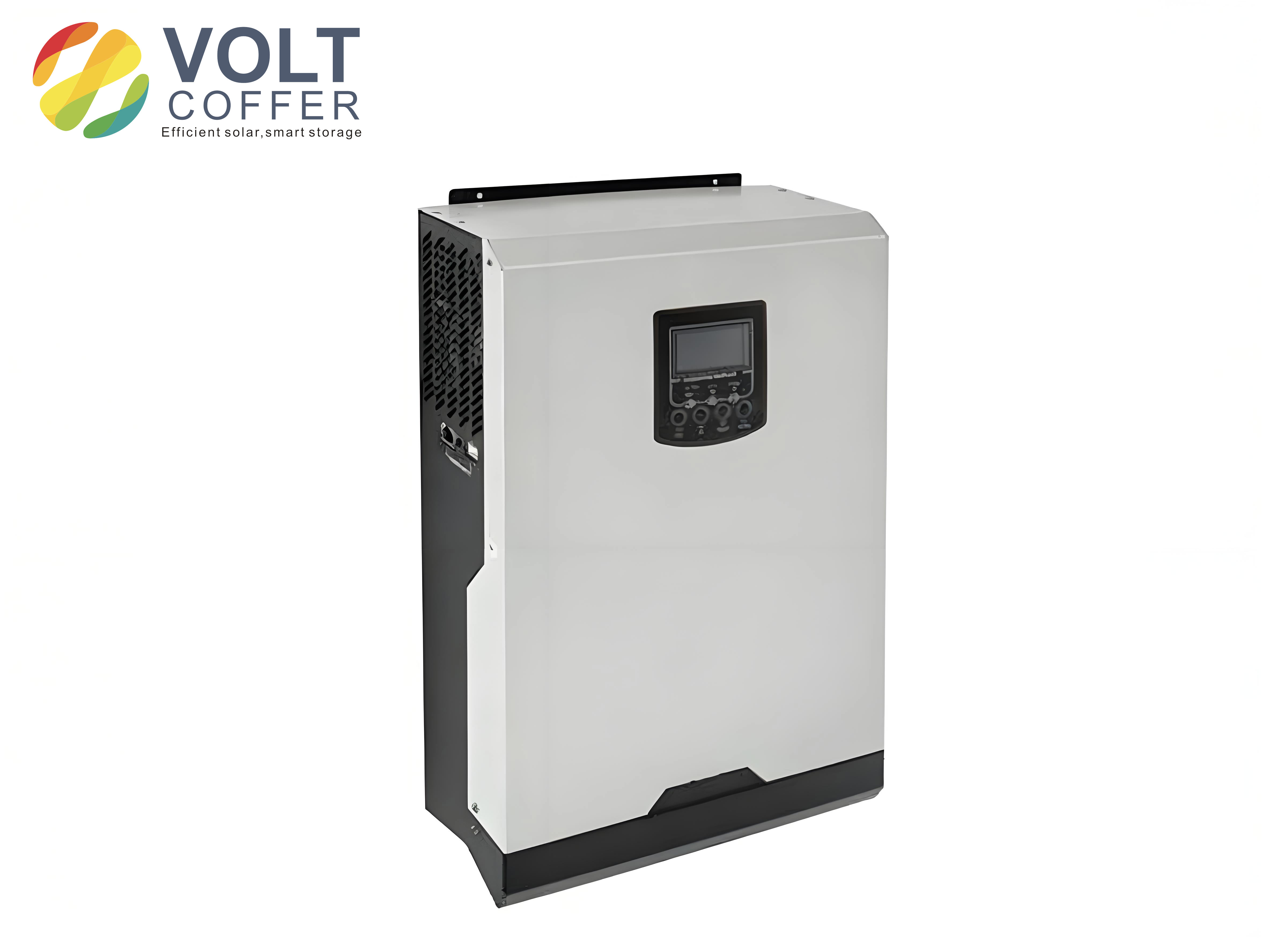
The main circuit parameter design is critical for efficiency, stability, and current quality. I designed the boost inductor to keep the converter in continuous conduction mode. I also designed the direct-current bus capacitor to limit voltage ripple and to provide energy buffering between the boost stage and the inverter stage. For the alternating-current side, I used an LC filter to attenuate switching harmonics and to produce a nearly sinusoidal grid current. The filter inductance and capacitance were selected so that the resonant frequency is far above the fundamental frequency and far below the switching frequency.
For the boost converter, the inductor current increment during the on-time is
$$
\Delta I_L(+) = \frac{V_s}{L} D_c T_s
$$
and the inductor current decrement during the off-time is
$$
\Delta I_L(-) = \frac{V_o – V_s}{L} (1-D_c) T_s
$$
Under steady-state operation, these two increments are equal, and the voltage gain is
$$
M = \frac{V_o}{V_s} = \frac{1}{1-D_c}
$$
The critical inductance for continuous conduction mode is
$$
L \ge \frac{V_o^2 T_s}{27 P_o}
$$
Using a direct-current bus voltage of 400 V, a switching period of 50 microseconds, and an output power of 3000 W, I found that the minimum inductance is about 0.198 mH. I selected a larger value with margin to reduce current ripple and to improve stability.
The direct-current bus capacitor was selected from the voltage ripple requirement. The capacitor value is
$$
C \ge \frac{P_o D_c T_s}{V_o \Delta V_o}
$$
With a voltage ripple below one percent of the bus voltage and a maximum duty cycle of 0.75, the minimum capacitance was about 70 microfarads. Because the capacitor also provides energy buffering, I used a much larger effective capacitance in the prototype.
For the alternating-current filter, I used two inductors and one capacitor. The maximum current ripple is approximately
$$
\Delta i \le \frac{V_{dc} T_s}{4(L_1+L_2)}
$$
and I required this ripple to be between ten and twenty percent of the rated alternating current. Therefore, the total inductance must satisfy
$$
L_1+L_2 \ge \frac{V_{dc} T_s}{(10\%\sim20\%) 4 I_{ac}}
$$
The resonant frequency of the filter is
$$
f_L = \frac{1}{2\pi \sqrt{(L_1+L_2)C}}
$$
I selected the filter so that the resonant frequency is much higher than 50 Hz and much lower than the 20 kHz switching frequency. The transfer function of the filter, including the equivalent load resistance, can be written as
$$
G(S) = \frac{1}{(L_1+L_2)C S^2 + R C S + 1}
$$
With a total inductance of about 2 mH, a capacitance of about 5 microfarads, and an equivalent load resistance of about 16.13 ohms, the filter provides strong attenuation of the switching frequency while introducing only a very small phase delay at the fundamental frequency. The attenuation at 20 kHz is substantial, and the phase delay at 50 Hz is about 1.45 degrees.
| Parameter | Value | Design Basis |
|---|---|---|
| Rated output power | 3 kW | Prototype rating |
| Direct-current bus voltage | 400 V | Above grid peak voltage |
| Boost switching frequency | 20 kHz | Acceptable loss and filter size |
| Boost inductance | 1 mH or higher | Continuous conduction margin |
| Direct-current bus capacitance | Effective value above 1.5 mF | Voltage ripple and energy buffering |
| Filter total inductance | About 2 mH | Current ripple limitation |
| Filter capacitance | About 5 microfarads | Harmonic attenuation and reactive power |
| Grid frequency | 50 Hz | Utility grid |
| Grid voltage | 220 V root mean square | Single-phase utility |
The control framework of my solar inverter includes maximum power point tracking, sinusoidal pulse-width modulation, dual-loop control, grid phase locking, and islanding detection. The boost stage is controlled to track the maximum power point of the photovoltaic array, while the inverter stage is controlled to regulate the direct-current bus voltage and to inject a sinusoidal current into the grid. The voltage outer loop generates a current amplitude reference, and the current inner loop forces the actual grid current to follow this reference. A grid-voltage feedforward term is added to the current loop to reduce the influence of grid voltage disturbances and to improve dynamic response.
| Control Function | Implementation Stage | Main Purpose |
|---|---|---|
| Maximum power point tracking | Boost converter | Extract maximum photovoltaic power |
| Direct-current bus voltage regulation | Inverter voltage outer loop | Balance photovoltaic power and grid power |
| Grid current regulation | Inverter current inner loop | Track sinusoidal current reference |
| Sinusoidal pulse-width modulation | Inverter bridge | Generate switching pulses |
| Grid synchronization | Capture interrupt and phase-locked loop | Match grid phase and frequency |
| Anti-islanding protection | Capture interrupt and detection algorithm | Disconnect when grid is lost |
The photovoltaic cell model is based on the photovoltaic effect of a semiconductor p-n junction. Under constant irradiance, the cell behaves approximately as a current source in parallel with a diode and a shunt resistance, with a series resistance representing internal losses. The output current can be expressed as
$$
I = I_L – I_o \left( e^{\frac{q(V+IR_s)}{nkT}} – 1 \right) – \frac{V+IR_s}{R_{sh}}
$$
where \(I_L\) is the photogenerated current, \(I_o\) is the reverse saturation current, \(q\) is the electron charge, \(k\) is the Boltzmann constant, \(T\) is the absolute temperature, \(n\) is the diode ideality factor, \(R_s\) is the series resistance, and \(R_{sh}\) is the shunt resistance. For practical simulation, I used a simplified model with short-circuit current, open-circuit voltage, maximum power point current, and maximum power point voltage. The simplified current-voltage relation is
$$
I = I_{sc} \left[ 1 – A \left( e^{\frac{V}{B V_{oc}}} – 1 \right) \right]
$$
where the intermediate coefficients are
$$
A = \left( 1 – \frac{I_m}{I_{sc}} \right) e^{-\frac{V_m}{B V_{oc}}}
$$
and
$$
B = \left( \frac{V_m}{V_{oc}} – 1 \right) \left[ \ln \left( 1 – \frac{I_m}{I_{sc}} \right) \right]^{-1}
$$
I also included irradiance and temperature effects. The photocurrent changes with irradiance and temperature, while the open-circuit voltage decreases as temperature rises. The current variation and voltage variation can be approximated by temperature coefficients. The resulting current-voltage and power-voltage curves show a clear nonlinear behavior. For a given irradiance and temperature, there is a unique maximum power point. When irradiance increases, the short-circuit current and maximum power increase. When temperature increases, the open-circuit voltage and maximum power decrease slightly.
| Condition | Effect on Short-Circuit Current | Effect on Open-Circuit Voltage | Effect on Maximum Power |
|---|---|---|---|
| Irradiance increases | Increases significantly | Increases slightly | Increases significantly |
| Irradiance decreases | Decreases significantly | Decreases slightly | Decreases significantly |
| Temperature increases | Increases slightly | Decreases | Decreases |
| Temperature decreases | Decreases slightly | Increases | Increases |
| Partial shading | May create multiple steps | May create multiple peaks | May create multiple local maxima |
Maximum power point tracking is essential for solar inverters because the photovoltaic output is nonlinear and strongly dependent on environmental conditions. I studied several algorithms, including constant-voltage control, perturbation and observation, incremental conductance, fuzzy logic control, and neural-network prediction. Constant-voltage control is simple but inaccurate when temperature and irradiance change. Fuzzy logic and neural-network methods can be fast but require complex implementation and tuning. I focused on perturbation and observation, incremental conductance, and a scanning method combined with incremental conductance.
The principle of perturbation and observation is to perturb the operating voltage periodically and to observe the resulting change in power. If the power increases, the next perturbation continues in the same direction. If the power decreases, the perturbation direction is reversed. The algorithm is simple and easy to implement, and it performs well when irradiance changes slowly. However, the perturbation step size creates a trade-off between tracking speed and steady-state oscillation. A large step gives fast tracking but causes power oscillation around the maximum power point. A small step reduces oscillation but slows the response. Under rapidly changing irradiance, the algorithm can make an incorrect decision and lose the maximum power point temporarily.
The incremental conductance method uses the derivative of power with respect to voltage. At the maximum power point, the derivative is zero, so
$$
\frac{dP}{dV} = I + V \frac{dI}{dV} = 0
$$
which gives the condition
$$
\frac{dI}{dV} = -\frac{I}{V}
$$
If the conductance increment is greater than the negative instantaneous conductance, the operating voltage should be increased. If it is smaller, the operating voltage should be decreased. If the two sides are equal, the maximum power point has been reached. The incremental conductance method provides more accurate tracking and smaller steady-state oscillation than perturbation and observation. It also responds better to changing irradiance and temperature. Its main disadvantage is the need for accurate current and voltage derivatives, which requires sufficient sampling resolution and computational speed.
For partial shading conditions, the power-voltage curve can have multiple peaks. A conventional incremental conductance method may converge to the first local peak and miss the global maximum. I therefore considered a scanning method combined with incremental conductance. The scanning method first tracks a local peak, records its power, then moves the operating voltage to a new region and tracks another peak. After scanning several regions, the algorithm compares the recorded peak powers and selects the global maximum. This method improves energy capture under partial shading, but it requires more memory and computation.
| Algorithm | Tracking Speed | Steady-State Oscillation | Implementation Complexity | Partial Shading Performance |
|---|---|---|---|---|
| Constant voltage | Fast | Low | Very low | Poor |
| Perturbation and observation | Moderate | Moderate to high | Low | Poor to moderate |
| Incremental conductance | Fast | Low | Moderate | Moderate |
| Scanning plus incremental conductance | Moderate | Low | High | Good |
| Fuzzy logic | Fast | Low | High | Moderate |
| Neural network | Fast | Low | Very high | Moderate to good |
I simulated the photovoltaic model and the boost converter with the perturbation and observation method and the incremental conductance method. The simulation results showed that both methods can reach the maximum power point quickly under standard irradiance and temperature. The incremental conductance method produced a smoother power waveform, smaller oscillation around the maximum power point, and better transition when irradiance changed from 1 kW/m² to 1.1 kW/m². I therefore selected incremental conductance as the main maximum power point tracking algorithm, with the scanning extension reserved for partial shading conditions.
The inverter stage uses sinusoidal pulse-width modulation. The basic idea is to compare a sinusoidal reference with a triangular carrier. The pulse widths are proportional to the sinusoidal reference, so the fundamental component of the output voltage approximates a sine wave. The modulation index is
$$
M = \frac{U_r}{U_c}
$$
and the carrier ratio is
$$
N = \frac{f_c}{f_r}
$$
I used unipolar sinusoidal pulse-width modulation because it produces fewer harmonics than bipolar modulation and because it is compatible with the H6 bridge. In the unipolar scheme, the output voltage switches between zero and the positive bus voltage during the positive half-cycle, and between zero and the negative bus voltage during the negative half-cycle. The output filter then removes the high-frequency components.
For the implementation, I considered natural sampling, regular sampling, and direct area equivalent methods. Natural sampling gives high accuracy but requires solving a transcendental equation, which is not suitable for real-time digital control. Regular sampling is simple and suitable for digital implementation. The on-time in regular sampling is
$$
T_{on} = T_c M \sin \omega t
$$
which can be written as
$$
T_{on} = \frac{T_c M}{N} \sin \left( \frac{2\pi k}{N} \right)
$$
where \(k\) is the sampling index. The direct area equivalent method calculates pulse widths so that each pulse area equals the corresponding area under the sine wave. Its pulse width is
$$
d = \frac{M}{\omega} \left[ \cos \left( \frac{2\pi k}{N} \right) – \cos \left( \frac{2\pi (k+1)}{N} \right) \right]
$$
This method gives a waveform very close to a sine wave, but it requires more computation. In my digital signal processor implementation, I used a practical combination of regular sampling and area-equivalent correction to balance accuracy and computational load.
The proportional-integral controller is used in both the voltage outer loop and the current inner loop. The continuous-time proportional-integral control law is
$$
u(t) = K_p e(t) + \frac{1}{T_I} \int_0^t e(t) dt
$$
where \(K_p\) is the proportional gain, \(T_I\) is the integral time constant, and \(e(t)\) is the control error. The discrete form is
$$
u(k) = K_p e(k) + K_i \sum_{j=0}^{k} e(j)
$$
For digital implementation, I used the incremental form
$$
\Delta u(k) = u(k) – u(k-1) = K_p [e(k)-e(k-1)] + K_i e(k)
$$
The incremental form avoids the accumulation of all past errors, reduces computational load, and limits the effect of a single faulty sample. I also applied limits to the error and to the output so that the duty cycle and current reference remain within safe bounds.
The dual-loop control structure contains a voltage outer loop and a current inner loop. The voltage outer loop regulates the direct-current bus voltage. The measured bus voltage is compared with a reference value, and the error is processed by a proportional-integral controller. The output of this controller becomes the amplitude reference for the grid current. This amplitude is multiplied by a unit sine wave synchronized with the grid voltage to produce the current reference. The current inner loop compares the actual grid current with this reference, and its proportional-integral controller generates the modulation signal for sinusoidal pulse-width modulation.
The current inner loop can be represented by the open-loop transfer function
$$
G_I(S) = G_P(S) G_{INV}(S) G_L(S)
$$
where \(G_P(S)\) is the proportional-integral controller, \(G_{INV}(S)\) is the inverter transfer function, and \(G_L(S)\) is the filter transfer function. When the grid voltage is considered as a disturbance, the transfer function becomes
$$
G_I'(S) = (G_P(S) G_{INV}(S) – U_{net}) G_L(S)
$$
To cancel the grid voltage disturbance, I added a grid-voltage feedforward term. The improved transfer function is
$$
G_I”(S) = (G_P(S) G_{INV}(S) + G_{fd}(S) U_{net} G_{INV}(S) – U_{net}) G_L(S)
$$
For perfect compensation, the feedforward function should be
$$
G_{fd}(S) = \frac{1}{G_{INV}(S)}
$$
The feedforward path makes the modulation signal follow the grid voltage closely and reduces the burden on the current controller. It also helps maintain a reasonable duty cycle when the direct-current bus voltage is only slightly higher than the grid voltage peak. In my design, the bus voltage was set to 400 V, while the grid peak voltage was about 311 V, so the duty cycle remained in a safe range.
| Loop | Controlled Variable | Reference | Output | Main Challenge |
|---|---|---|---|---|
| Voltage outer loop | Direct-current bus voltage | 400 V | Current amplitude reference | Balancing photovoltaic power and grid power |
| Current inner loop | Grid current | Sinusoidal current reference | Modulation signal | Fast tracking and low harmonic distortion |
| Feedforward path | Grid voltage | Measured grid voltage | Compensation signal | Rejecting grid voltage disturbance |
Islanding detection is another key function of solar inverters. Islanding occurs when the utility grid is disconnected but the solar inverter continues to supply power to local loads. This condition is dangerous because it can endanger maintenance personnel and because it can cause voltage and frequency instability. Passive detection methods monitor voltage amplitude, frequency, and harmonics. They are simple but have a non-detection zone. Active detection methods intentionally introduce a small disturbance into the output current or frequency. When the grid is connected, the grid absorbs the disturbance. When the grid is disconnected, the disturbance accumulates and quickly exceeds a threshold, allowing detection.
The islanding equivalent model includes a parallel RLC load connected to the solar inverter and the grid. Under normal operation, the active and reactive power balance is
$$
P = P_{load} + \Delta P
$$
and
$$
Q = Q_{load} + \Delta Q
$$
The load active power is
$$
P_{load} = \frac{U_a^2}{R}
$$
and the load reactive power is
$$
Q_{load} = \left( \omega C – \frac{1}{\omega L} \right) U_a^2
$$
When the grid is lost, the active and reactive power supplied by the grid become zero. If the local load power exactly matches the inverter output power, the voltage and frequency may not change, creating a non-detection zone. Active frequency drift is an effective way to reduce this zone. In my implementation, I shifted the inverter output frequency by a small amount, such as 0.02 Hz, and increased the shift gradually if the grid frequency did not follow. When the grid was connected, the grid held the frequency stable. When the grid was disconnected, the frequency drifted until it exceeded the allowed range, and the inverter disconnected from the load.
I simulated the active frequency drift method with a parallel RLC load. The grid switch opened at 0.5 s. After islanding occurred, the current and voltage waveforms decayed to zero within about 0.04 s, and the relay opened. This confirmed that the method can detect islanding quickly and reliably. I combined this active method with passive over-voltage, under-voltage, over-frequency, and under-frequency protection to improve overall safety.
| Detection Method | Principle | Advantages | Limitations |
|---|---|---|---|
| Over-voltage and under-voltage | Monitor voltage amplitude | Simple and fast | Non-detection zone when power matches |
| Over-frequency and under-frequency | Monitor frequency | Simple and fast | Non-detection zone when reactive power matches |
| Harmonic detection | Monitor harmonic distortion | No disturbance | Sensitive to grid background harmonics |
| Active frequency drift | Introduce frequency disturbance | Small non-detection zone | Slightly degrades current quality |
| Active power perturbation | Introduce power disturbance | Effective for active power mismatch | Affects maximum power tracking |
For hardware implementation, I selected a digital signal processor from the TMS320F28035 family. This device has a 32-bit fixed-point core, a 60 MHz clock, and an instruction cycle of about 16.67 ns. It includes enhanced pulse-width modulation modules, a 12-bit analog-to-digital converter, capture modules, and communication peripherals. The enhanced pulse-width modulation module can generate complex pulse patterns with minimal central processing unit load. The analog-to-digital converter has multiple channels and can be triggered by the pulse-width modulation module, which is important for synchronous sampling of the grid voltage and current.
| Hardware Block | Function | Reason for Selection |
|---|---|---|
| Digital signal processor | Main control and algorithm execution | Fast arithmetic and integrated peripherals |
| Enhanced pulse-width modulation | Generate switching pulses | High resolution and flexible event control |
| Analog-to-digital converter | Sample voltages and currents | 12-bit resolution and fast conversion |
| Capture module | Detect grid zero crossings | Accurate phase and frequency measurement |
| Communication peripherals | Monitoring and external interface | Supports system integration |
The signal detection circuits convert high-voltage and high-current signals into low-voltage signals suitable for the analog-to-digital converter. For direct-current voltage, I used a resistor divider followed by a buffer and a limiting circuit. For direct-current current, I used a Hall-effect current sensor. For alternating-current grid voltage and current, I used differential amplifier circuits with filtering and a direct-current bias to shift the signal into the 0 to 3.3 V range. I also used a zero-crossing comparator to detect the grid voltage phase. The comparator output was conditioned and fed to the capture module.
The analog-to-digital converter in the digital signal processor can have gain and offset errors. I corrected these errors by applying two known reference voltages to two channels and reading the corresponding digital values. The ideal conversion relationship is
$$
ADC_{Result} = \frac{Input – V_{REFLO}}{3.3} \times 4096
$$
Using two known input-output pairs, I calculated the gain and offset correction coefficients and applied them to all other channels. This improved the accuracy of the current and voltage measurements and reduced harmonic distortion in the grid current.
Because the sampling circuits contain RC filters, the sampled alternating-current signals lag the actual signals. I therefore applied a predictive algorithm to compensate for the delay. If \(Q_1\), \(Q_2\), \(Q_3\), and \(Q_4\) are four consecutive samples, the predicted value can be written as
$$
Q_n = Q_4 + (Q_4-Q_3) + \frac{1}{2}(Q_4 – 2Q_3 + Q_2) + \frac{1}{6}(Q_4 – 3Q_3 + 3Q_2 – Q_1)
$$
which simplifies to
$$
Q_n = \frac{8}{3}Q_4 – \frac{5}{2}Q_3 + Q_2 – \frac{1}{6}Q_1
$$
I also used a first-order inertial filter with an anti-interference threshold. If the difference between the new sample and the previous filtered value exceeded a limit, the new sample was replaced by the previous filtered value. This suppressed random spikes without slowing the response too much.
The software was organized around a main loop and several interrupt service routines. The main loop performed initialization of the input-output ports, system clock, enhanced pulse-width modulation module, capture module, analog-to-digital converter channels, and interrupt controllers. After initialization, the main loop waited for interrupts. The pulse-width modulation interrupt ran at 20 kHz and performed analog-to-digital sampling, filtering, maximum power point tracking, sinusoidal pulse-width modulation calculation, proportional-integral control, and protection checks. The capture interrupt handled grid phase locking, frequency measurement, and active frequency drift for islanding detection.
| Software Module | Execution Rate | Main Tasks |
|---|---|---|
| Main loop | Continuous | Initialization and background monitoring |
| Pulse-width modulation interrupt | 20 kHz | Sampling, filtering, MPPT, current control, protection |
| Capture interrupt | Grid zero crossing | Phase locking, frequency measurement, anti-islanding |
| Analog-to-digital correction | Startup or periodic | Gain and offset compensation |
| Communication | Asynchronous | Monitoring and parameter adjustment |
The phase-locking algorithm records the grid voltage phase at each zero crossing and compares it with the phase of the sinusoidal modulation reference. The difference is used to adjust the phase pointer of the modulation wave. In this way, the grid current remains in phase with the grid voltage. I used a capture interrupt to measure the grid period and to calculate the frequency. If the frequency deviated beyond the allowed range, the inverter stopped and disconnected from the grid.
The start-up and grid-connection sequence was designed to be safe and orderly. First, the digital signal processor initialized all peripherals and checked the photovoltaic voltage and current. If the photovoltaic voltage was sufficient, the boost converter started and raised the direct-current bus voltage. The duty cycle was limited to prevent over-voltage. When the bus voltage reached the required value, the inverter checked the grid voltage amplitude, phase, and frequency. After successful synchronization, the relay closed and the inverter began to inject current. The maximum power point tracking function then adjusted the boost duty cycle to extract the maximum available photovoltaic power. Throughout operation, the controller monitored bus voltage, grid voltage, grid current, and frequency. If any fault was detected, the relay opened and the converter stopped.
| Start-Up Step | Action | Safety Check |
|---|---|---|
| 1 | Initialize digital signal processor and peripherals | Clock and memory self-test |
| 2 | Check photovoltaic voltage and current | Minimum voltage and maximum current |
| 3 | Start boost converter | Duty-cycle limit and bus voltage limit |
| 4 | Check grid voltage, phase, and frequency | Amplitude, phase, and frequency window |
| 5 | Close relay and begin current injection | Inrush current and synchronization check |
| 6 | Enable maximum power point tracking | Power change and voltage limit |
| 7 | Monitor faults continuously | Over-current, over-voltage, islanding |
I built a 3 kW prototype to validate the design. The prototype accepted a maximum photovoltaic input power of 3500 W, a maximum direct-current input voltage of 500 V, and an input current of 0 to 20 A. The maximum power point tracking voltage range was 200 to 400 V. The direct-current bus voltage was set to 400 V. The sinusoidal pulse-width modulation carrier frequency was 20 kHz, and the modulation frequency followed the grid at 50 Hz with a tolerance of plus or minus 2.5 Hz. The output voltage was 230 V with a tolerance of plus or minus ten percent, and the grid current was rated at up to 16.5 A. I used an oscilloscope, digital multimeter, current probe, programmable alternating-current source, and load bank for testing.
| Prototype Parameter | Value |
|---|---|
| Maximum photovoltaic input power | 3500 W |
| Maximum direct-current input voltage | 500 V |
| Input current range | 0 to 20 A |
| Maximum power point tracking voltage range | 200 to 400 V |
| Direct-current bus voltage | 400 V |
| Switching frequency | 20 kHz |
| Grid frequency | 50 Hz plus or minus 2.5 Hz |
| Output voltage | 230 V plus or minus ten percent |
| Grid current | 0 to 16.5 A |
In the direct-current sampling tests, the photovoltaic voltage was divided down to a small voltage within the analog-to-digital converter range. The digital signal processor reconstructed the actual voltage using a scaling factor. The bus voltage and photovoltaic current were processed in the same way. The measured waveforms confirmed that the sampling circuits provided stable signals for the control algorithms.
For grid phase detection, I compared the grid voltage with the zero-crossing comparator output. The comparator produced a square wave with an edge near the grid voltage zero crossing. I observed a small phase lag of about 8.57 degrees, which I compensated in the software by adjusting the phase pointer when the edge was detected. This ensured that the current reference remained aligned with the grid voltage.
The full-bridge drive waveforms showed the expected unipolar sinusoidal pulse-width modulation pattern. The two line-frequency switches operated at 50 Hz, while the high-frequency switches operated at 20 kHz. The inverter output voltage and current were filtered by the LC network and delivered to the grid. The maximum power point tracking test showed that the operating point moved quickly to the maximum power point on the power-voltage curve. The measured maximum power point tracking efficiency was above 99 percent, which validated the incremental conductance algorithm and the boost control strategy.
The grid-connected voltage and current waveforms showed that the current was in phase with the voltage under medium and high power conditions. At low power, the current amplitude was small, and the sampling resolution and noise became more significant, which caused some waveform distortion. At higher power, the current was smoother and the power factor was close to unity, although some harmonics remained. These harmonics can be reduced by improving the filter design, increasing the sampling resolution, and fine-tuning the proportional-integral gains.
| Test Item | Observed Result | Interpretation |
|---|---|---|
| Photovoltaic voltage sampling | Stable scaled signal | Voltage sensing circuit works correctly |
| Grid zero-crossing detection | Small phase lag of about 8.57 degrees | Software compensation required |
| Full-bridge drive | Unipolar pulse-width modulation pattern | H6 bridge operates as designed |
| Maximum power point tracking | Efficiency above 99 percent | Incremental conductance method is effective |
| Grid current at low power | Some distortion due to small signal amplitude | Resolution and noise limit performance |
| Grid current at high power | In phase with voltage, moderate harmonics | Dual-loop control works but can be improved |
The experimental results confirmed that the two-stage solar inverter architecture, the incremental conductance maximum power point tracking method, the unipolar sinusoidal pulse-width modulation, the dual-loop control with grid-voltage feedforward, and the active frequency drift anti-islanding method can work together in a practical prototype. The prototype reached the expected power level and maintained stable operation during grid connection. The direct-current bus voltage remained close to its reference, and the grid current followed the reference with acceptable accuracy. The maximum power point tracking efficiency was high, and the islanding detection responded quickly when the grid was disconnected.
I also identified several areas for improvement. The boost converter experiences switching losses during turn-on and turn-off. Adding a soft-switching network could reduce these losses and improve efficiency. The maximum power point tracking algorithm could be extended to handle partial shading more effectively. The scanning method combined with incremental conductance was studied in simulation, but its full implementation in the prototype requires more memory and more careful tuning. The grid current harmonics could be reduced by optimizing the filter parameters, increasing the controller resolution, and using a more accurate phase-locked loop. At low power, the current distortion was more noticeable, so future work should focus on improving small-signal measurement accuracy and on adaptive gain scheduling.
| Improvement Area | Problem | Proposed Action |
|---|---|---|
| Boost converter loss | Switching loss during turn-on and turn-off | Add soft-switching network |
| Partial shading | Multiple local power peaks | Implement scanning plus incremental conductance |
| Grid current harmonics | Residual harmonics at medium and high power | Optimize filter and tune current loop |
| Low-power distortion | Small signal amplitude and noise | Improve sampling resolution and gain scheduling |
| Islanding detection | Prototype implementation requires further tuning | Refine active frequency drift and passive thresholds |
| System integration | Communication and monitoring are basic | Add advanced monitoring and fault diagnosis |
In summary, I designed and tested a single-phase grid-connected solar inverter for photovoltaic applications. I selected a boost plus H6 full-bridge topology, derived the main circuit parameters, developed a photovoltaic model, compared maximum power point tracking algorithms, implemented sinusoidal pulse-width modulation and proportional-integral control, added grid-voltage feedforward, studied anti-islanding detection, and built a 3 kW prototype. The experimental results showed that the solar inverter can track the maximum power point with high efficiency and inject current into the grid with acceptable power quality. The work provides a practical foundation for further development of more efficient, more reliable, and more intelligent solar inverters.
I believe that solar inverters will continue to evolve toward higher frequency, smaller size, lower cost, and greater intelligence. Modular micro-inverters are especially promising because they can be distributed across individual photovoltaic panels, improving energy harvest under partial shading and simplifying system expansion. Digital signal processors and advanced control algorithms will make it possible to integrate maximum power point tracking, grid synchronization, anti-islanding protection, fault diagnosis, and communication into a single compact unit. With continued research and development, solar inverters will play an increasingly important role in the transition to a clean and sustainable energy system.