
The rapid growth of renewable energy has made the solar panel one of the most important components in modern power systems. Solar cells convert sunlight directly into electricity, but their fragile silicon structure may be damaged during manufacturing, transportation, installation, and outdoor operation. These damages often appear as defects such as finger interruption, cracks, black cores, fragments, and thick lines. Since defects directly reduce the power generation efficiency of a solar panel, robust and efficient defect detection is essential. In this work, I focus on machine-vision-based defect detection algorithms for solar panel electroluminescence (EL) images. I first construct a well-annotated defect dataset, then improve the YOLOv8 model from two directions: high accuracy and lightweight deployment. The work is organized around a high-precision model and a lightweight model, both designed to meet the practical requirements of industrial solar panel quality inspection.
1. Introduction and Motivation
In the past decade, photovoltaic power generation has become increasingly competitive. The global transition toward clean energy creates a growing demand for reliable solar panel products. However, the core component of a photovoltaic system, the solar cell, is very fragile. Defects can occur at any stage of production and use. EL imaging is a widely used technique for inspecting solar cells because it can reveal internal defects through the radiative recombination of carriers. In an EL image, areas with defects often appear darker or exhibit unusual patterns. Figure 1 below shows a typical outdoor solar panel installation scene that motivates the need for automated visual inspection.
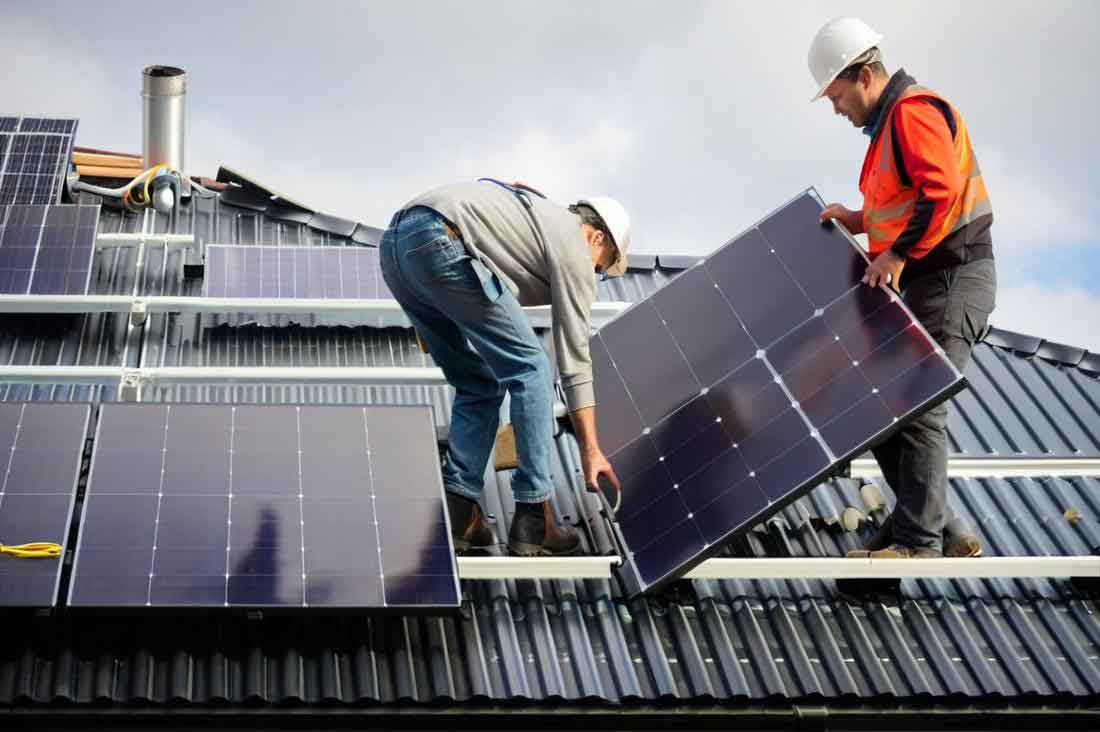
Manual inspection is time-consuming and error-prone. Traditional physical methods, such as ultrasound, X-ray, and thermography, require expensive equipment and specialized knowledge. With the advances in deep learning, object detection algorithms have shown great potential for automated defect detection. Among them, YOLO (You Only Look Once) is one of the most popular families. YOLOv8, in particular, offers a good trade-off between speed and accuracy. Nevertheless, standard YOLOv8 still has limitations when applied to solar panel EL images. The uneven brightness, complex background, small defect size, and high similarity between defects make detection difficult. Therefore, I propose several targeted improvements to YOLOv8.
2. Related Work
2.1 Traditional and Physical Inspection Methods
Early inspection of solar panel defects mainly relied on human eyes. This method is subjective and inefficient. Later, physical detection techniques were developed. For example, resonance ultrasonic vibration can identify cracks in silicon wafers. Electrically loaded thermography detects defects by measuring temperature differences caused by power loss. Infrared cameras can locate hot spots and broken solder joints. Although these methods are useful, their hardware cost and operating complexity prevent widespread adoption in online quality control.
2.2 Machine Vision and Deep Learning Methods
Machine vision approaches usually capture images first and then apply image processing or machine learning algorithms. Image processing methods include edge detection, threshold segmentation, Fourier transform, and morphological analysis. These methods work well for some specific defects but often fail to generalize. Deep learning methods, especially convolutional neural networks (CNNs), have become dominant. CNNs automatically learn hierarchical features from raw images. Two-stage detectors such as Faster R-CNN offer high accuracy but slow speed. One-stage detectors such as YOLO are much faster and are preferred in real-time industrial inspection.
2.3 YOLOv8 Architecture
YOLOv8 is the latest YOLO model from Ultralytics. Its structure consists of a backbone, a neck, and a detection head. The backbone extracts features using Conv modules, C2f modules, and a SPPF module. The neck applies Feature Pyramid Network (FPN) and Path Aggregation Network (PAN) to fuse multi-scale features. The head is anchor-free and decouples classification from regression. The loss function contains classification loss, CIoU loss, and Distribution Focal Loss. YOLOv8 has several model sizes: n, s, m, l, and x. In this work, I choose YOLOv8n as the baseline because of its small size and high efficiency.
Convolution is the fundamental operation of a CNN. Given an input image matrix \(X \in \mathbb{R}^{M \times N}\) and a kernel \(W \in \mathbb{R}^{U \times V}\), the discrete convolution is defined as:
$$Y_{ij} = \sum_{u=1}^{U} \sum_{v=1}^{V} W_{uv} X_{i-u+1, j-v+1}$$
Compared with fully connected layers, convolutional layers have two important properties: sparse interaction and parameter sharing. Sparse interaction means each neuron only connects to a local region of the previous layer. Parameter sharing means the same kernel is reused across all spatial positions. These properties greatly reduce the number of parameters.
3. Build the Solar Panel Defect Dataset
3.1 Data Description
The original dataset used in this study is a public industrial detection dataset produced by EL imaging. It contains infrared images of solar cells with various defects and heterogeneous backgrounds. I select four common defect categories: finger interruption, linear crack, star crack, and thick line. The original dataset has 2718 images. The number of samples in each category is extremely unbalanced. For instance, the star crack category has only about one hundred samples while the finger interruption category has more than two thousand. This imbalance severely limits model training.
3.2 Data Augmentation and Annotation
To solve the small-sample problem, I use two approaches. First, I apply data augmentation to the star crack images. I use the Albumentations library to perform random brightness and contrast adjustment, rotation, vertical flip, and horizontal flip. These operations produce more diverse images and help the model generalize better. Second, I manually label additional unlabeled star crack defects using the Make Sense annotation tool. The annotation results are stored in XML files and then converted into YOLO-format TXT files. Each line of the TXT file contains the class index and normalized bounding box coordinates. After preprocessing, the total number of images increases to 3230. The final sample counts are: 3102 finger samples, 1508 linear crack samples, 846 star crack samples, and 993 thick line samples.
3.3 Comparison Before and After Preprocessing
To verify the effectiveness of the preprocessing, I train YOLOv8n on both the original and preprocessed datasets. The results are shown in the following table.
| Dataset | Precision | Recall | mAP@50 | mAP@50:95 |
|---|---|---|---|---|
| Before preprocessing | 0.833 | 0.788 | 87.2% | 53.2% |
| After preprocessing | 0.894 | 0.809 | 88.2% | 56.2% |
| Improvement | +6.1% | +2.1% | +1.0% | +3.0% |
From the table, the preprocessing improves all evaluation metrics. The precision increases by 6.1%, recall increases by 2.1%, mAP@50 increases from 87.2% to 88.2%, and mAP@50:95 increases from 53.2% to 56.2%. This demonstrates that data augmentation and manual annotation are useful for solar panel defect detection.
4. High-Accuracy YOLOv8 Algorithm
To improve the accuracy of defect detection, I propose a model named YOLOv8-SPW. The name stands for YOLOv8-SGE-PConv-WIoU. The model introduces three modifications to YOLOv8n: a Spatial Group-wise Enhance (SGE) attention mechanism, a variant of Partial Convolution (PConv), and the Wise-IoU (WIoU) loss function. These modifications address the problems of background interference, feature diversity, and sample quality imbalance.
4.1 SGE Attention Mechanism
SGE is a lightweight attention module that can enhance semantic features by grouping channels. Given a feature map \(\mathbf{X}\) with \(C\) channels, SGE divides it into \(G\) groups. Each group contains \(m = H \times W\) spatial feature vectors:
$$\mathbf{x}_i \in \mathbb{R}^{\frac{C}{G}}, \quad i=1,2,\dots,m$$
For each group, SGE calculates a global semantic vector by global average pooling:
$$\mathbf{g} = \frac{1}{m} \sum_{i=1}^{m} \mathbf{x}_i$$
Then, the correlation between each local feature and the global semantic vector is computed by dot product:
$$c_i = \mathbf{g} \cdot \mathbf{x}_i$$
These coefficients are normalized with the mean and standard deviation of \(c\):
$$\hat{c}_i = \frac{c_i – \mu_c}{\sigma_c + \epsilon}$$
Next, a learnable scale and shift are applied:
$$a_i = \gamma \hat{c}_i + \beta$$
Finally, the original feature is scaled by the sigmoid function:
$$\hat{\mathbf{x}}_i = \mathbf{x}_i \cdot \sigma(a_i)$$
This mechanism helps the network focus on important spatial regions and suppress noise. In my high-accuracy model, I add SGE to the neck network. The neck fuses semantic and location information, so SGE is beneficial in selecting the most relevant features. The following table shows the comparison of SGE placement.
| Model | Finger AP | Crack AP | Star crack AP | Thick line AP | mAP@50 | mAP@50:95 | Params/M |
|---|---|---|---|---|---|---|---|
| YOLOv8n | 0.951 | 0.774 | 0.914 | 0.889 | 88.2% | 56.2% | 6.3 |
| +SGE backbone | 0.937 | 0.784 | 0.940 | 0.901 | 89.1% | 56.5% | 6.3 |
| +SGE neck | 0.939 | 0.824 | 0.932 | 0.912 | 90.2% | 56.7% | 6.3 |
The table shows that adding SGE in the neck improves mAP@50 from 88.2% to 90.2%. The parameter count remains unchanged at 6.3M. This proves that SGE is very efficient and beneficial for solar panel defect detection.
4.2 Variant PConv Module
Partial Convolution (PConv) is a new convolution operation introduced in FasterNet. It applies convolution only on a subset of channels to reduce redundant computation. Given an input feature map with \(C\) channels, PConv applies standard convolution on the first \(c_p\) channels and keeps the remaining channels unchanged. The output is then concatenated with the unchanged channels. When \(c_p = C/4\), the FLOPs of PConv become:
$$\text{FLOPs}_{\text{PConv}} = H \times W \times K^2 \times c_p = H \times W \times K^2 \times \frac{C}{4}$$
For a standard convolution with the same input and output channels, the FLOPs are:
$$\text{FLOPs}_{\text{Conv}} = H \times W \times K^2 \times C$$
Thus, PConv requires only one sixteenth of the FLOPs of standard convolution. In my variant, I add a Conv module after the concatenation operation. The structure can be represented as:
$$\mathbf{y} = \text{Conv}\left(\text{Concat}\left(\text{PConv}(\mathbf{x}), \mathbf{x}_{\text{res}}\right)\right)$$
This variant increases feature diversity. The Conv module applies batch normalization and a nonlinear activation function, allowing the network to learn more complex feature representations. I insert the variant PConv after C2f modules in the neck. The experimental results are shown below.
| Model | Finger AP | Crack AP | Star crack AP | Thick line AP | mAP@50 | mAP@50:95 | Params/M |
|---|---|---|---|---|---|---|---|
| YOLOv8n | 0.951 | 0.774 | 0.914 | 0.889 | 88.2% | 56.2% | 6.3 |
| +PConv backbone | 0.945 | 0.802 | 0.912 | 0.900 | 89.0% | 56.8% | 6.5 |
| +PConv neck | 0.944 | 0.822 | 0.946 | 0.900 | 90.3% | 56.9% | 6.5 |
Adding PConv in the neck improves mAP@50 by 2.1% and mAP@50:95 by 0.7%. The parameter count increases slightly from 6.3M to 6.5M, but the accuracy gain is significant. This makes the variant PConv a suitable module for solar panel defect detection.
4.3 Wise-IoU Loss
The original YOLOv8 uses CIoU as the regression loss. CIoU considers overlap area, center distance, and aspect ratio. However, CIoU applies a fixed penalty mechanism and does not sufficiently handle low-quality samples. To address this, I replace CIoU with WIoU. WIoU designs a wise focusing weight to balance different sample qualities.
The first version WIoU-v1 is defined as:
$$L_{\text{WIoUv1}} = R_{\text{WIoU}} \cdot L_{\text{IoU}}$$
where
$$R_{\text{WIoU}} = \exp\left(\frac{(x – x_{gt})^2 + (y – y_{gt})^2}{W_g^2 + H_g^2}\right)$$
and
$$L_{\text{IoU}} = 1 – \text{IoU}$$
Here, \(W_g\) and \(H_g\) are the width and height of the minimum bounding box, and \(x,y\) are the center coordinates of the predicted box. WIoU-v2 adds a monotonic focusing coefficient:
$$L_{\text{WIoUv2}} = L_{\text{IoU}}^{\gamma^*} \cdot L_{\text{WIoUv1}}$$
WIoU-v3 introduces a non-monotonic focusing coefficient based on the outlier degree \(\beta\):
$$\beta = \frac{L_{\text{IoU}}}{\bar{L}_{\text{IoU}}}$$
and
$$r = \frac{\beta}{\delta \alpha^{\beta – \delta}}$$
Then:
$$L_{\text{WIoUv3}} = r \cdot L_{\text{WIoUv1}}$$
I evaluate all three versions of WIoU. The results are shown in the following table.
| Regression Loss | Finger AP | Crack AP | Star crack AP | Thick line AP | mAP@50 | mAP@50:95 |
|---|---|---|---|---|---|---|
| CIoU | 0.951 | 0.774 | 0.914 | 0.889 | 88.2% | 56.2% |
| WIoU-v1 | 0.941 | 0.834 | 0.920 | 0.896 | 89.8% | 56.6% |
| WIoU-v2 | 0.940 | 0.794 | 0.898 | 0.896 | 88.2% | 56.5% |
| WIoU-v3 | 0.947 | 0.805 | 0.902 | 0.905 | 89.0% | 57.6% |
WIoU-v1 gives the highest mAP@50, reaching 89.8%. WIoU-v3 achieves the best mAP@50:95 at 57.6%. Since my goal is to improve overall detection accuracy, I choose WIoU-v1 as the regression loss for the final model.
4.4 Ablation Study of High-Accuracy Model
To verify the contribution of each module, I conduct an ablation study. The experiment starts from YOLOv8n and gradually adds SGE, PConv, and WIoU. The results are shown below.
| SGE | PConv | WIoU | mAP@50 | mAP@50:95 |
|---|---|---|---|---|
| 88.2% | 56.2% | |||
| Yes | 90.2% | 56.7% | ||
| Yes | 90.3% | 56.9% | ||
| Yes | 89.8% | 56.6% | ||
| Yes | Yes | 90.7% | 57.6% | |
| Yes | Yes | Yes | 91.0% | 57.8% |
The combination of all three modules gives the best performance. mAP@50 improves from 88.2% to 91.0%, and mAP@50:95 improves from 56.2% to 57.8%. This proves that the proposed high-accuracy model can effectively improve solar panel defect detection.
4.5 Comparison with Other High-Precision Models
I compare the YOLOv8-SPW model with YOLOv3, YOLOv5n-p6, YOLOv6n, YOLOv7, and original YOLOv8n. All models are trained under the same conditions. The comparison results are presented in the table below.
| Model | mAP@50 | mAP@50:95 | Params/M |
|---|---|---|---|
| YOLOv3 | 87.7% | 59.2% | 207.8 |
| YOLOv5n-p6 | 87.7% | 55.1% | 8.6 |
| YOLOv6n | 87.3% | 54.1% | 8.7 |
| YOLOv7 | 82.9% | 44.5% | 12.3 |
| YOLOv8n | 88.2% | 56.2% | 6.3 |
| YOLOv8-SPW | 91.0% | 57.8% | 6.3 |
YOLOv3 has a high mAP@50:95 but a huge parameter count. YOLOv8-SPW achieves the highest mAP@50 and a competitive mAP@50:95 while maintaining a small model size. Therefore, the high-accuracy model is suitable for industrial solar panel inspection.
5. Lightweight YOLOv8n Defect Detection Model
In many practical situations, defect detection equipment has limited computational resources. To satisfy real-time requirements, I design a lightweight model called YOLOv8n-ES. The name stands for YOLOv8n-EfficientNet-SGE. The main idea is to replace the original backbone with a compact EfficientNet architecture and add SGE attention to the neck.
5.1 EfficientNet Backbone
EfficientNet is a family of efficient CNN architectures that use compound scaling. The baseline network EfficientNet-B0 is built from repeated MBConv modules. The compound scaling method is:
$$d = \alpha^{\phi}, \quad w = \beta^{\phi}, \quad r = \gamma^{\phi}$$
with the constraint:
$$\alpha \cdot \beta^2 \cdot \gamma^2 \approx 2$$
Here, \(d\) is the depth scaling factor, \(w\) is the width scaling factor, and \(r\) is the resolution scaling factor. This method balances all dimensions of the network. In my lightweight model, I use EfficientNet-B0 as the backbone. The backbone consists of a 3×3 convolution layer followed by 16 MBConv blocks. MBConv uses depthwise separable convolution and the Squeeze-and-Excitation (SE) module. Depthwise separable convolution splits standard convolution into depthwise convolution and pointwise convolution. This greatly reduces the number of parameters.
The MBConv structure can be summarized as:
$$\mathbf{y} = \text{DropConnect}\left(\text{SE}\left(\text{DepthwiseConv}\left(\text{Conv}_{1\times 1}(\mathbf{x})\right)\right)\right)$$
By replacing the original YOLOv8n backbone, the model size decreases significantly. The parameter count drops from 6.3M to 4.1M. However, the accuracy also decreases slightly. To compensate for this loss, I introduce the SGE attention mechanism into the neck network.
5.2 SGE in the Lightweight Model
SGE is very lightweight and can be inserted into any part of the network. In the lightweight model, I add SGE to the feature fusion path after the FPN and PAN structure. This helps the model focus on important defect features and suppress irrelevant information. SGE is especially useful for small defect targets in solar panel EL images. The following table compares the performance before and after adding SGE.
| Model | Finger AP | Crack AP | Star crack AP | Thick line AP | mAP@50 | mAP@50:95 | Params/M | FPS |
|---|---|---|---|---|---|---|---|---|
| YOLOv8n | 0.951 | 0.774 | 0.914 | 0.889 | 88.2% | 56.2% | 6.3 | 72.9 |
| +EfficientNet | 0.941 | 0.789 | 0.891 | 0.876 | 87.4% | 55.3% | 4.1 | 70.6 |
| +EfficientNet+SGE | 0.952 | 0.808 | 0.931 | 0.880 | 89.3% | 57.1% | 4.1 | 79.9 |
The table shows that adding SGE improves mAP@50 from 87.4% to 89.3%, which is even higher than the original YOLOv8n. The FPS increases from 72.9 to 79.9, a 10% improvement. The parameter count remains at 4.1M. This result demonstrates that SGE can effectively enhance the detection ability of a lightweight network.
5.3 Ablation Study of Lightweight Model
I perform another ablation study to understand the contribution of the EfficientNet backbone and SGE module. The results are shown below.
| EfficientNet | SGE | mAP@50 | Params/M | FPS |
|---|---|---|---|---|
| 88.2% | 6.3 | 72.9 | ||
| Yes | 87.4% | 4.1 | 70.6 | |
| Yes | 90.2% | 6.3 | 78.5 | |
| Yes | Yes | 89.3% | 4.1 | 79.9 |
The combination of EfficientNet and SGE achieves the best FPS and a good accuracy. Compared with the baseline, the lightweight model reduces parameters by 35%, improves processing speed by about 10%, and increases mAP@50 by 1.1%. This makes YOLOv8n-ES a strong candidate for edge deployment in solar panel inspection systems.
5.4 Comparison with Other Lightweight Models
To further validate the lightweight model, I compare it with several YOLO lightweight versions:
| Model | mAP@50 | Params/M | FPS |
|---|---|---|---|
| YOLOv3-tiny | 85.0% | 24.4 | 76.3 |
| YOLOv5n | 88.4% | 5.3 | 77.9 |
| YOLOv7-tiny | 85.8% | 12.3 | 104.4 |
| YOLOv8n | 88.2% | 6.3 | 72.9 |
| YOLOv8n-ES | 89.3% | 4.1 | 79.9 |
YOLOv7-tiny has a higher FPS, but its parameter count is three times larger than YOLOv8n-ES. YOLOv5n has a low parameter count, but both mAP@50 and FPS are lower than YOLOv8n-ES. Therefore, YOLOv8n-ES provides a better trade-off among accuracy, speed, and model size. It is well suited for real-time solar panel defect detection on resource-limited devices.
6. Experimental Environment and Evaluation Metrics
All experiments are conducted on a Windows 11 machine with PyTorch 2.0.0 and Python 3.8. The GPU is an RTX 3090 with 24GB memory. The CPU is an Intel Xeon Gold 6330 with 14 vCPUs. The input image size is 640×640. The batch size is 32. I train all models for 150 epochs. The optimizer is SGD with an initial learning rate of 0.01 and momentum of 0.937.
The main evaluation metrics are precision, recall, mAP@50, and mAP@50:95. The definitions are listed below.
| Metric | Formula | Description |
|---|---|---|
| IoU | \(\frac{|A \cap B|}{|A \cup B|}\) | Measures the overlap between predicted and ground-truth boxes. |
| Precision | \(P = \frac{TP}{TP + FP}\) | Fraction of correctly predicted positive boxes among all predicted boxes. |
| Recall | \(R = \frac{TP}{TP + FN}\) | Fraction of correctly predicted positive boxes among all ground-truth boxes. |
| AP | \(\int_{0}^{1} P(R) dR\) | Area under the precision-recall curve. |
| mAP@50 | \(\frac{1}{N}\sum_{i=1}^{N} AP_i\) at IoU=0.5 | Mean average precision at IoU threshold 0.5. |
| mAP@50:95 | Average of mAP at IoU thresholds from 0.5 to 0.95 | Mean average precision averaged over multiple IoU thresholds. |
In addition to accuracy, I use the number of parameters and FPS to measure the efficiency of a model. Parameter count represents the model storage requirement. FPS measures the number of frames processed per second. A higher FPS indicates better real-time performance.
7. Discussion
Experimental results show that both proposed models improve the detection of defects in solar panel EL images. The high-accuracy model YOLOv8-SPW reaches 91.0% mAP@50 by combining SGE, PConv, and WIoU. The lightweight model YOLOv8n-ES reaches 89.3% mAP@50 while reducing the model size to 4.1M parameters. These results are valuable for industrial quality control.
One interesting finding is that the addition of SGE alone improves mAP@50 from 88.2% to 90.2% when added to the neck of YOLOv8n. In the lightweight model, SGE not only restores the accuracy lost by EfficientNet but also improves the FPS. This suggests that SGE can help the network make better use of compressed feature representations. Another finding is that WIoU-v1 is more stable than WIoU-v2 and WIoU-v3 in this defect detection task. The reason may be that the dataset contains many low-quality samples, and WIoU-v1 provides a balanced focusing mechanism without excessive penalty.
I also observe that replacing the backbone with EfficientNet reduces the parameter count but initially reduces accuracy. However, after adding SGE, the accuracy becomes higher than the original model. This demonstrates that a lightweight architecture can maintain high performance if the feature fusion part is well designed. The success of SGE in both the high-accuracy and lightweight models confirms its strong generalization capability.
The proposed methods still have limitations. For instance, all experiments are conducted on one public dataset. More defect types and more diverse environmental conditions should be considered in future work. Manual annotation is time-consuming and prone to errors. Automatic annotation or semi-supervised learning may help to reduce the labeling cost. In addition, the current models do not completely solve the false detection and missed detection problems. More advanced attention mechanisms or multi-scale fusion strategies may further improve performance.
8. Conclusion
In this work, I research machine-vision-based defect detection algorithms for solar panel EL images. I first build a complete dataset by data augmentation and manual annotation. The dataset contains four defect categories and 3230 images. Then, I propose a high-accuracy model YOLOv8-SPW. By introducing SGE attention, a variant PConv module, and WIoU loss, the model improves mAP@50 from 88.2% to 91.0%. The model does not increase the parameter count. Finally, I propose a lightweight model YOLOv8n-ES. This model replaces the original backbone with EfficientNet and adds SGE to the neck. The parameter count is reduced by 35%, the FPS is increased by about 10%, and mAP@50 is improved by 1.1%.
Both models have been verified through extensive experiments. The high-accuracy model is suitable for off-line or server-side inspection systems that require high precision. The lightweight model is suitable for edge devices and real-time quality control systems. The research results provide useful solutions for solar panel defect detection and can be extended to other industrial vision tasks.
Future Work
In the future, I plan to expand the dataset to include more defect types and larger-scale samples. I also want to explore automatic labeling methods to reduce manual effort. For the high-accuracy model, I will investigate more advanced loss functions and attention modules. For the lightweight model, I will study pruning and knowledge distillation to further reduce model size. I believe that machine vision will continue to play an important role in solar panel quality assurance.
Another promising direction is to integrate the detection algorithm into a complete industrial inspection system. Such a system should include image acquisition, defect detection, classification, and reporting. The lightweight model is especially suitable for embedded systems that operate in real time. With the rapid development of deep learning, the accuracy and speed of solar panel defect detection will continue to improve.
In summary, this thesis presents two effective algorithms based on YOLOv8. The high-accuracy model and the lightweight model both outperform the baseline on the constructed solar panel defect dataset. The proposed methods contribute to the field of machine vision and provide practical guidance for solar panel manufacturing and maintenance.