
Photovoltaic (PV) power generation has become one of the most important renewable energy sources worldwide. With the rapid expansion of PV plants, the reliability and efficiency of solar panels are increasingly challenged by various defects that occur during long-term outdoor operation. These defects, such as hot spots, bypass diode faults, cracks, bird droppings, and dust accumulation, can significantly degrade the performance of solar panels and even lead to safety hazards. Traditional manual inspection methods are labor-intensive, subjective, and unsuitable for large-scale PV plants. To address these issues, I have developed an intelligent defect detection system based on deep learning, which leverages both infrared and visible-light images captured by drones. In this article, I describe the complete research pipeline, including dataset construction, semantic segmentation of solar panel regions, two dedicated object detection algorithms for internal and surface defects, and a graphical user interface for practical deployment.
Solar panel defect detection has drawn considerable attention from both academia and industry. Early approaches relied on manually designed feature extraction rules, which required expert knowledge and were only applicable to specific defect types. Subsequently, traditional machine learning methods, such as support vector machines and neural networks, improved detection performance but still depended on handcrafted features and lacked robustness in complex backgrounds. Recently, deep learning has revolutionized the field by automatically learning hierarchical features from raw images. Convolutional neural networks and transformer-based architectures have achieved remarkable success in object detection and semantic segmentation, enabling accurate and efficient solar panel defect identification. However, existing algorithms often fail to balance detection accuracy, model size, and computational cost, especially when deployed on resource-constrained drone platforms. Therefore, my research focuses on developing lightweight yet accurate deep learning models tailored to solar panel inspection tasks.
The remainder of this article is organized as follows. First, I describe the construction of infrared and visible-light datasets for solar panel defects, along with data augmentation strategies. Then, I present an improved semantic segmentation network for extracting solar panel regions from infrared images, which effectively suppresses false detections caused by similar backgrounds. Next, I introduce two advanced object detection algorithms: one for internal defects detected in infrared images, and another for surface defects detected in visible-light images. Finally, I demonstrate the implementation of a complete defect detection system with a user-friendly interface, followed by conclusions and future directions.
Dataset Construction and Augmentation
To train and evaluate deep learning models for solar panel defect detection, I constructed two separate datasets: an internal defect dataset and a surface defect dataset. The internal defect dataset contains 2,585 infrared images of solar panels, annotated with two classes: hot spots and bypass diode faults. The surface defect dataset contains 3,246 visible-light images, annotated with three classes: cracks, bird droppings, and dust accumulation. All images were collected from public datasets and uncrewed aerial vehicle (UAV) captures under various lighting conditions, angles, and altitudes. The diversity of the data ensures that the trained models generalize well to real-world inspection scenarios.
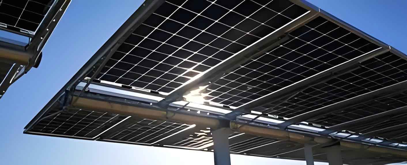
Infrared imaging is particularly suitable for detecting internal thermal defects because defective regions often exhibit higher temperatures due to abnormal energy dissipation. For example, hot spots arise when solar cells are partially shaded or damaged, causing reverse bias and localized heating. Bypass diode faults, on the other hand, produce a characteristic bright rectangular band across the solar panel, covering one-third or two-thirds of its area. Visible-light imaging is more effective for surface defects, as cracks appear as dense white lines, bird droppings as small spot-like or elongated stains, and dust as a uniform reduction in surface reflectivity. These distinct characteristics guided the design of my detection algorithms.
Since the original number of images was insufficient for training deep networks and could lead to overfitting, I applied data augmentation techniques to increase the diversity and quantity of the datasets. Specifically, I used random brightness adjustment, random rotation, and random flipping. Brightness adjustment emulates different illumination conditions by varying pixel intensities by ±25%. Rotation randomly rotates images by angles in the range of −90° to +90°, using a rotation matrix as follows:
$$ R(\theta) = \begin{bmatrix} \cos\theta & -\sin\theta \\ \sin\theta & \cos\theta \end{bmatrix} $$
Flipping includes horizontal and vertical mirror operations, which further enrich the training set. After augmentation, the number of samples increased as shown in the following tables. The augmented datasets were then split into training, validation, and test sets with a ratio of 7:2:1. All annotations were stored in PASCAL VOC format, which can be easily converted to COCO or YOLO formats for different network models.
| Internal defect class | Original images | Augmented images |
|---|---|---|
| Hot spot | 1,497 | 2,158 |
| Bypass diode fault | 1,169 | 1,865 |
| Surface defect class | Original images | Augmented images |
| Bird droppings | 1,397 | 2,037 |
| Crack | 1,128 | 1,836 |
| Dust | 867 | 1,596 |
The use of augmented data significantly improved the robustness of my models. Training with a large and diverse dataset helps the network learn invariant features and reduces the risk of overfitting, which is essential for deployment in complex field environments.
Semantic Segmentation of Solar Panel Regions
One major challenge in infrared-based solar panel defect detection is that the background often looks very similar to the solar panels. For instance, the ground under strong sunlight may appear as bright regions that resemble hot spots, leading to false positives. To eliminate this problem, I first segment the solar panel region from the infrared image before performing defect detection. Semantic segmentation assigns a class label to every pixel, allowing me to extract only the solar panel area and discard irrelevant background.
I chose the U-Net architecture as the baseline because of its excellent performance in medical image segmentation and its ability to work well with limited training data. However, the original U-Net has a relatively large number of parameters, which is undesirable for embedded drone applications. Moreover, its segmentation boundaries are often blurry under varying illumination and temperature conditions. To overcome these limitations, I proposed an improved model named CM2Unet, which consists of three main components: a segmentation branch, an edge detection branch, and a feature fusion module.
The encoder of the U-Net is replaced by MobileNetV2, a lightweight backbone network that significantly reduces the parameter count while preserving strong feature extraction capabilities. MobileNetV2 employs inverted residual blocks and linear bottlenecks. The inverted residual block first expands the input to a higher dimension using 1×1 convolution, then applies depthwise convolution for spatial feature extraction, and finally projects back to a lower dimension. This structure improves gradient flow and reduces computation. The basic blocks are illustrated in the following equations. For a stride of 1, the block uses the inverted residual structure with a shortcut connection. For stride 2, the shortcut is removed because the spatial dimensions change.
$$ y = \begin{cases} \mathcal{B}(x) + x, & \text{if stride}=1 \\ \mathcal{B}(x), & \text{if stride}=2 \end{cases} $$
Here, \(\mathcal{B}(x)\) represents the composed operations of 1×1 expansion, depthwise convolution, batch normalization, ReLU6 activation, and 1×1 projection. By leveraging MobileNetV2, the number of parameters of my CM2Unet is only 6.83 million, which is less than one-fourth of the original U-Net (31.38 million).
The edge detection branch uses the Canny algorithm to generate edge maps of the input image. The Canny algorithm performs Gaussian smoothing, gradient magnitude computation, non-maximum suppression, and double thresholding. The gradient magnitude is computed as:
$$ M(i,j) = \sqrt{P_x(i,j)^2 + P_y(i,j)^2} $$
where \(P_x\) and \(P_y\) are the partial derivatives in the horizontal and vertical directions, respectively. The edge map highlights the boundaries of solar panels, which is crucial for accurate segmentation.
The fusion module combines the high-level semantic features from the encoder with the edge information from the edge detection branch. First, the edge feature map passes through 2×2 convolution and pooling layers to adjust its resolution and extract higher-order features. Then, the encoded features and the edge features are concatenated along the channel dimension. A 1×1 convolution is used to reduce the number of channels and ensure spatial alignment. The fused features are fed into the decoder, which progressively upsamples them to the original image resolution. This design forces the network to pay extra attention to boundary regions, resulting in sharper and more accurate segmentation masks.
I trained the CM2Unet on the infrared solar panel dataset with labels created using the Labelme tool. The training setup included an input size of 640×640, a batch size of 16, an initial learning rate of 0.01, and 300 epochs. The model was implemented in PyTorch and trained on an NVIDIA RTX 3080 Ti GPU with 12 GB memory. To evaluate the segmentation performance, I used the mean Intersection over Union (MIoU) metric, defined as:
$$ \text{MIoU} = \frac{1}{n+1}\sum_{i=0}^{n} \frac{p_{ii}}{\sum_{j=0}^{n} p_{ij} + \sum_{j=0}^{n} p_{ji} – p_{ii}} $$
where \(p_{ij}\) represents the number of pixels of class \(i\) predicted as class \(j\). A higher MIoU indicates better alignment between the predicted mask and the ground truth. I compared CM2Unet with several mainstream segmentation networks, including DeepLabv3+, SegNet, ENet, SQNet, FPENet, and the original U-Net. The results are summarized in the following table.
| Model | MIoU (%) | Parameters (M) |
|---|---|---|
| DeepLabv3+ | 93.22 | 43.51 |
| SegNet | 93.65 | 29.45 |
| ENet | 81.63 | 0.36 |
| SQNet | 83.97 | 1.27 |
| FPENet | 83.62 | 0.52 |
| U-Net | 94.65 | 31.38 |
| CM2Unet | 97.38 | 6.83 |
As shown, my proposed CM2Unet achieved the highest MIoU of 97.38%, which is 2.73 percentage points higher than the original U-Net and significantly better than other networks. In terms of parameter count, CM2Unet is much lighter than DeepLabv3+ and SegNet, while maintaining acceptable model size compared to the most lightweight networks. Visual inspection of the segmentation results confirmed that my method effectively suppresses background interference and produces clean, continuous boundaries even in scenarios with complex backgrounds or discontinuous solar panels. The integration of edge information and MobileNetV2 features proved to be highly beneficial for accurate solar panel region extraction.
Internal Defect Detection with IN-PV-YOLO
After extracting the solar panel region, the next step is to detect internal defects in infrared images. The internal defect detection task faces several challenges: defects have large scale variations (small hot spots vs. large bypass diode fault areas), high similarity among different defect types, and complex thermal patterns. Moreover, the algorithm must be lightweight enough to run on drones. To address these challenges, I proposed IN-PV-YOLO, a modified YOLOv8n model that balances accuracy and computational efficiency.
YOLOv8n is the smallest version of the YOLOv8 family, consisting of a backbone, a neck, and a head. The backbone uses a convolutional neural network with CSP and C2f modules to extract multi-scale features. The neck uses a path aggregation network (PAFPN) to fuse features from different levels, and the head predicts bounding boxes and class probabilities. While YOLOv8n is already relatively lightweight, its accuracy on solar panel defects is insufficient. I therefore introduced four major improvements.
First improvement: lightweight backbone with VanillaNet. The original backbone of YOLOv8n is replaced by VanillaNet, an extremely simple yet effective architecture that only uses 1×1 convolutions and pooling layers. VanillaNet consists of a stem that downsamples the input, followed by several stages that gradually increase the number of channels while reducing spatial dimensions through max or average pooling. The final stage produces the classification output. This design dramatically reduces computational cost and parameters. The GFLOPs of the backbone drop from 8.1 to 5.0, and the parameter count drops from 3.01M to 1.73M, without sacrificing accuracy.
Second improvement: DBoTNet feature extraction layer. The original SPPF module is replaced by a novel DBoTNet (Double Bottleneck Transformer) layer. BoTNet integrates global multi-head self-attention (MHSA) into a residual bottleneck block. In each block, the 3×3 spatial convolution is replaced by a multi-head self-attention module. The operation can be expressed as:
$$ \text{Attention}(Q,K,V) = \text{softmax}\left(\frac{QK^T}{\sqrt{C}}\right) V $$
where \(Q\), \(K\), and \(V\) are the query, key, and value matrices obtained by linear transformations of the input feature map. In my DBoTNet, I process the features from two parallel branches through the same bottleneck transformer module before concatenating them. This dual-branch design improves feature consistency and stability, leading to better detection accuracy. As a result, the model gains the ability to capture long-range dependencies and global context, which is crucial for distinguishing defects with similar appearances.
Third improvement: fused receptive field attention. To enhance feature extraction, I designed a new attention mechanism called RFCBAM (Receptive Field Convolutional Block Attention Module). This module combines receptive field spatial attention with channel attention. Unlike standard CBAM, which performs channel and spatial attention separately, RFCBAM uses group convolutions to extract spatial features from the receptive field and applies a squeeze-and-excitation style channel attention without average pooling. The structure allows the network to assign different weights to features from different positions, overcoming the parameter sharing limitation of standard convolutions. I used RFCBAM to improve both the convolution layers and the C2f bottlenecks. The improved C2f module, named C2f_RFCBAM, replaces the original bottleneck blocks with RFCBAM-based blocks. This yields a significant improvement in precision and recall with only a negligible increase in parameters.
Fourth improvement: V7DownSampling module. To handle the varying sizes of defects, I introduced the V7DownSampling module, which combines max pooling with multiple convolution branches. The module downsamples the spatial resolution while merging features from different scales. It effectively enlarges the receptive field and helps the network detect objects of different sizes. I applied this module in both the backbone and the neck, specifically at the P3, P5, P7 stages in the backbone and P17, P20 stages in the neck. This architecture enables efficient multi-scale fusion and reduces computation.
Fifth improvement: Focaler-WIoU loss function. The default YOLOv8n uses CIoU loss, which has limitations due to the ambiguous aspect ratio. I adopted Focaler-WIoU, which combines the dynamic focusing mechanism of Wise-IoU with linear interval mapping from Focaler-IoU. The Focaler-IoU loss is defined as:
$$ L_{\text{Focaler-IoU}} = 1 – \text{IoU}_{\text{Focaler}} $$
where
$$ \text{IoU}_{\text{Focaler}} = \begin{cases} 0, & \text{IoU} < d \\ \frac{\text{IoU} – d}{u – d}, & d \le \text{IoU} \le u \\ 1, & \text{IoU} > u \end{cases} $$
By adjusting the parameters \(d\) and \(u\), the loss focuses on different regression samples. The final combined loss is:
$$ L_{\text{Focaler-WIoU}} = L_{\text{WIoUv3}} + \text{IoU}_{\text{Focaler}} – \text{IoU} $$
This loss function enables the model to learn more informative gradients and improves bounding box regression accuracy.
The complete IN-PV-YOLO architecture is shown conceptually in the following table, which summarizes the key components.
| Component | Details |
|---|---|
| Backbone | VanillaNet + V7DownSampling |
| Neck | C2f_RFCBAM + DBoTNet + V7DownSampling |
| Head | YOLOv8 detection head |
| Loss | Focaler-WIoU |
I conducted extensive experiments on the internal defect dataset. The evaluation metrics included precision (P), recall (R), mean average precision at IoU=0.5 (mAP50), GFLOPs, and parameter count. Ablation studies were performed by adding each improvement step by step to the baseline. The results are shown in the table below.
| Method | GFLOPs | P (%) | R (%) | mAP50 (%) | Params (M) |
|---|---|---|---|---|---|
| YOLOv8n | 8.1 | 68.2 | 70.7 | 70.9 | 3.01 |
| +VanillaNet | 5.0 | 68.1 | 71.2 | 71.3 | 1.73 |
| +RFCBAM | 8.8 | 68.4 | 72.9 | 72.9 | 3.15 |
| +V7DownSampling | 7.8 | 69.9 | 72.5 | 73.7 | 2.74 |
| +DBoTNet | 8.2 | 69.8 | 71.7 | 72.5 | 3.08 |
| +Focaler-WIoU | 8.1 | 68.7 | 72.5 | 72.5 | 3.01 |
| All improvements | 6.0 | 72.7 | 72.5 | 75.5 | 1.92 |
The final IN-PV-YOLO achieved a mAP of 75.5%, which is 4.6 percentage points higher than the baseline, while the GFLOPs decreased from 8.1 to 6.0 and the parameters decreased from 3.01M to 1.92M. This demonstrates that my improvement strategy simultaneously enhances accuracy and reduces model complexity. I also compared the proposed attention mechanism with other popular attention mechanisms, including RFA, MLCA, and CBAM. The results are listed below.
| Attention Mechanism | GFLOPs | mAP50 (%) | Params (M) |
|---|---|---|---|
| RFA | 8.8 | 72.2 | 3.13 |
| MLCA | 8.1 | 71.5 | 3.01 |
| CBAM | 8.1 | 71.7 | 3.02 |
| RFCBAM | 8.8 | 72.9 | 3.15 |
Furthermore, I compared the Focaler-WIoU loss with other common losses.
| Loss Function | mAP50 (%) |
|---|---|
| CIoU | 70.9 |
| ShapeIoU | 69.3 |
| SIoU | 71.7 |
| EIoU | 71.2 |
| GIoU | 69.4 |
| Focaler-WIoU | 72.5 |
To verify the generalization ability of my modifications, I applied the same improvement strategy to YOLOv8s and YOLOv8m. The results in the next table show consistent gains across different model scales.
| Model | P (%) | R (%) | mAP50 (%) | GFLOPs | Params (M) |
|---|---|---|---|---|---|
| YOLOv8n | 68.2 | 70.7 | 70.9 | 8.1 | 3.01 |
| YOLOv8n-ours | 72.7 | 72.5 | 75.5 | 6.0 | 1.92 |
| YOLOv8s | 76.9 | 73.5 | 78.2 | 28.4 | 11.13 |
| YOLOv8s-ours | 77.9 | 75.0 | 80.2 | 25.2 | 8.75 |
| YOLOv8m | 78.5 | 75.1 | 79.9 | 78.7 | 25.84 |
| YOLOv8m-ours | 81.0 | 76.5 | 82.1 | 70.5 | 22.35 |
Additionally, I compared IN-PV-YOLO with other mainstream object detection models. The results are shown below.
| Model | GFLOPs | Params (M) | mAP50 (%) |
|---|---|---|---|
| SSD | 62.8 | 26.29 | 59.2 |
| Faster R-CNN | 370.42 | 137.10 | 65.5 |
| YOLOv5n | 7.1 | 2.50 | 69.2 |
| YOLOv6n | 11.8 | 4.23 | 63.1 |
| YOLOv3-tiny | 18.9 | 12.13 | 57.4 |
| YOLOv3 | 282.2 | 103.67 | 82.7 |
| IN-PV-YOLO | 6.0 | 1.92 | 75.5 |
Although YOLOv3 achieves higher accuracy, its enormous computational cost and parameter count make it impractical for drone deployment. My IN-PV-YOLO offers the best trade-off between accuracy and efficiency. The training curves showed that the model converges quickly, with loss and mAP stabilizing after approximately 200 epochs. The visualization of detection results demonstrated that my model accurately detects hot spots and bypass diode faults while avoiding false positives caused by background structures.
Surface Defect Detection with SF-PV-YOLO
Visible-light images provide rich color and texture information, which is beneficial for identifying surface defects such as cracks, bird droppings, and dust. However, these defects exhibit large variations in size, shape, and orientation, and the background can be complex. To achieve high detection accuracy for surface defects, I proposed SF-PV-YOLO. Unlike the internal defect detector, which emphasizes lightweight design, the surface defect detector focuses more on accuracy, though it still maintains a reasonable model size for practical use.
The first major improvement is replacing the backbone with HGNetv2. HGNetv2 is a high-performance GPU-friendly network that uses hierarchical graph blocks. The architecture begins with an HGStem that performs initial downsampling through convolutional layers and max pooling. Then, several HGBlocks are stacked to extract features at multiple scales. Each HGBlock contains multiple convolutional branches with different kernel sizes, allowing the network to capture diverse features. Between blocks, a learnable downsampling layer reduces spatial dimensions while increasing channels. Finally, global average pooling produces the classification output. By employing HGNetv2, the backbone can effectively extract both low-level and high-level features, improving the representation capability for defects with varying sizes and shapes.
The second improvement is replacing the neck with an Attentional Feature Pyramid Network (AFPN). A conventional PAFPN suffers from semantic degradation when deep features pass through many intermediate layers. AFPN introduces adaptive feature fusion modules, called ASFF (Attentional Scale Sequence Fusion), to better combine features from different levels. For a two-level fusion (ASFF-2), the model performs upsampling or downsampling to align feature maps and then applies learned weights to fuse them. For a three-level fusion (ASFF-3), more complex alignment steps are used. The adaptive weighting is computed by:
$$ \alpha^{l}_{ij} = \frac{e^{\lambda^{l}_{ij}}}{\sum_{k} e^{\lambda^{k}_{ij}}} $$
where \(\lambda^{l}_{ij}\) are learnable parameters for level \(l\). This mechanism allows the network to dynamically balance contributions from different layers, thereby enhancing multi-scale detection performance.
The third improvement is the integration of a parameter-free attention mechanism, SPA (Swift Parameter-free Attention), into the C2f modules. SPA uses symmetric activation functions and residual connections to emphasize important features without adding learnable parameters. This is particularly attractive because it improves performance without increasing model size. The SPA-based C2f module, named C2f_SPAB, consists of several SPAB (SPA blocks) that extract features via three convolutions with a residual connection. The attention map is generated by a symmetric activation function applied to the extracted features. The final output is obtained by element-wise multiplication of the feature map and the attention map.
The fourth improvement is using depthwise separable convolutions instead of standard convolutions in certain parts of the network. Depthwise separable convolution splits a standard convolution into a depthwise convolution, which applies a single filter per input channel, and a pointwise convolution, which combines the output channels using 1×1 convolutions. The parameter count for a standard convolution is \(K_h \times K_w \times C_{in} \times C_{out}\), while for depthwise separable convolution it is \(K_h \times K_w \times C_{in} + C_{in} \times C_{out}\). This results in a significant reduction in parameters, making the model lighter.
I conducted ablation experiments to verify each improvement. The results are summarized below.
| Method | GFLOPs | P (%) | R (%) | mAP50 (%) | Params (M) |
|---|---|---|---|---|---|
| YOLOv8n | 8.1 | 68.6 | 63.5 | 66.4 | 3.01 |
| +HGNetv2 | 7.7 | 73.6 | 66.7 | 69.5 | 2.50 |
| +AFPN | 11.1 | 72.4 | 61.8 | 67.4 | 2.74 |
| +DWConv | 6.9 | 69.1 | 64.5 | 66.9 | 2.44 |
| +SPA | 8.2 | 70.8 | 63.6 | 67.6 | 3.02 |
| +HGNetv2+AFPN | 10.4 | 74.6 | 66.6 | 70.3 | 2.42 |
| +HGNetv2+AFPN+DWConv | 9.2 | 75.1 | 67.3 | 71.2 | 2.36 |
| All improvements | 9.3 | 75.9 | 68.2 | 72.1 | 2.53 |
The final SF-PV-YOLO model achieved a mAP of 72.1%, which is 5.7 percentage points higher than the baseline YOLOv8n, with only a modest increase in GFLOPs (from 8.1 to 9.3) and a decrease in parameters (from 3.01M to 2.53M). This demonstrates that the accuracy-oriented improvements are effective and efficient.
I also compared different attention mechanisms integrated into YOLOv8n for surface defect detection. The SPA attention achieved the best mAP with the smallest increase in parameters, as shown in the next table.
| Method | GFLOPs | P (%) | R (%) | mAP50 (%) | Params (M) |
|---|---|---|---|---|---|
| YOLOv8n | 8.1 | 68.6 | 63.5 | 66.4 | 3.01 |
| +SE | 8.3 | 67.9 | 67.7 | 67.2 | 3.05 |
| +CBAM | 8.3 | 70.5 | 62.2 | 67.3 | 3.11 |
| +SA | 8.6 | 70.2 | 63.1 | 66.9 | 3.52 |
| +SPA | 8.2 | 70.8 | 63.6 | 67.6 | 3.02 |
Visualization of detection results indicated that SF-PV-YOLO successfully detects cracks, bird droppings, and dust with high confidence and accurate localization. Compared to the baseline, the improved model significantly reduces false negatives and false positives, especially in scenarios with cluttered backgrounds or partially obscured defects.
System Design and Implementation
Based on the developed deep learning models, I designed and implemented a complete photovoltaic panel defect detection system. The system is built using Python, PyCharm, and Qt Designer, with a graphical user interface that allows users to interactively perform defect detection. The software includes several functional modules: user registration and login, function selection, image upload, solar panel segmentation, internal defect detection, and surface defect detection.
The login interface ensures secure access to the system. New users must register an account before logging in. After successful login, the user enters the main selection interface, where they can choose between “Surface Defect Detection” and “Internal Defect Detection”. The surface defect detection interface supports loading visible-light images via a file browser or online from a drone connection. The user can select the detection model: YOLOv8, YOLOv3, or the proposed SF-PV-YOLO. Once the detection is complete, the system displays the annotated image with bounding boxes, class labels, confidence scores, and positions.
The internal defect detection interface includes two stages. First, the user can choose a segmentation model (DeepLabv3+, U-Net, or CM2Unet) to extract the solar panel region from an infrared image. The segmented result is shown in the interface. Then, the user selects a detection model (YOLOv8, YOLOv3, or IN-PV-YOLO) to detect internal defects such as hot spots and bypass diode faults. The final output includes the defect types, confidence values, and relative coordinates. The system also provides a button to switch between the internal and surface detection interfaces, as well as a button to close the current page and return to the main menu.
I tested the system with representative images. For surface defects, the system correctly identified bird droppings, cracks, and dust. For internal defects, the system accurately segmented the solar panel region and successfully detected hot spots and bypass diode faults. The detection results were displayed in real time with high confidence. The system proved to be effective and user-friendly, meeting the requirements of practical photovoltaic plant inspection.
Conclusion and Future Work
In this research, I proposed a comprehensive deep learning-based solution for photovoltaic panel defect detection using UAV-acquired infrared and visible-light images. The main contributions are summarized as follows.
First, I developed an improved semantic segmentation network, CM2Unet, that combines MobileNetV2 and edge information to extract solar panel regions from infrared images. The model achieves a MIoU of 97.38% with only 6.83 million parameters, significantly reducing background false positives and improving segmentation accuracy. This preprocessing step is essential for reliable internal defect detection.
Second, I designed IN-PV-YOLO, a lightweight internal defect detector based on YOLOv8n. By incorporating VanillaNet, DBoTNet, RFCBAM attention, V7DownSampling, and Focaler-WIoU loss, the model achieves a mAP of 75.5% with only 6.0 GFLOPs and 1.92 million parameters. This detector is suitable for real-time processing on drones and provides accurate detection of hot spots and bypass diode faults.
Third, I proposed SF-PV-YOLO, an accuracy-oriented surface defect detector that uses HGNetv2, AFPN, SPA attention, and depthwise separable convolutions. The model achieves a mAP of 72.1% on the surface defect dataset, improving by 5.7 percentage points over the baseline while maintaining reasonable computational cost. This detector successfully identifies cracks, bird droppings, and dust in visible-light images.
Fourth, I implemented a user-friendly defect detection system using Qt Designer and Python. The system integrates all the proposed models and provides an interactive interface for uploading images, selecting models, and visualizing detection results. The system has been tested and validated on both internal and surface defect detection tasks.
Future work will focus on the following directions. First, I plan to further refine the detection algorithms to improve performance on similar and complex defects, such as distinguishing multiple hot spots from a bypass diode fault. Second, the dataset will be extended to include more defect types and more diverse environmental conditions, which will enhance the generalization capability of the models. Third, the system software will be optimized for real-time deployment on embedded platforms, such as Jetson devices, to enable onboard processing. Finally, I intend to incorporate multi-modal fusion of infrared and visible-light images to achieve a more comprehensive and robust defect diagnosis. These advancements will contribute to the intelligent operation and maintenance of photovoltaic power plants, ensuring higher efficiency and lower costs.