
In our recent research, we have developed a comprehensive deep learning framework for the classification and localization of defects in solar panels. The proposed system is designed to overcome the limitations of conventional manual inspection and single-image based detection approaches. By integrating advanced image stitching, segmentation, and convolutional neural network classification, our method can efficiently process aerial infrared images of large-scale photovoltaic plants and produce accurate defect maps. Throughout this paper, we emphasize the application of deep learning techniques for solar panel condition assessment, and we demonstrate the robustness of our algorithm under various real-world conditions.
The detection of defects in solar panels is critical for maintaining the efficiency and safety of photovoltaic power stations. Traditional manual inspection methods are time-consuming, costly, and often fail to detect subtle defects. In our work, we leverage unmanned aerial vehicles equipped with infrared cameras to capture local images of solar panel arrays. These images are then processed by our algorithm to generate a high-resolution panoramic view of the entire installation. Our approach not only identifies the exact location of defective solar panels but also classifies the type of defect, such as hot spots, diode failures, cracks, and normal conditions.
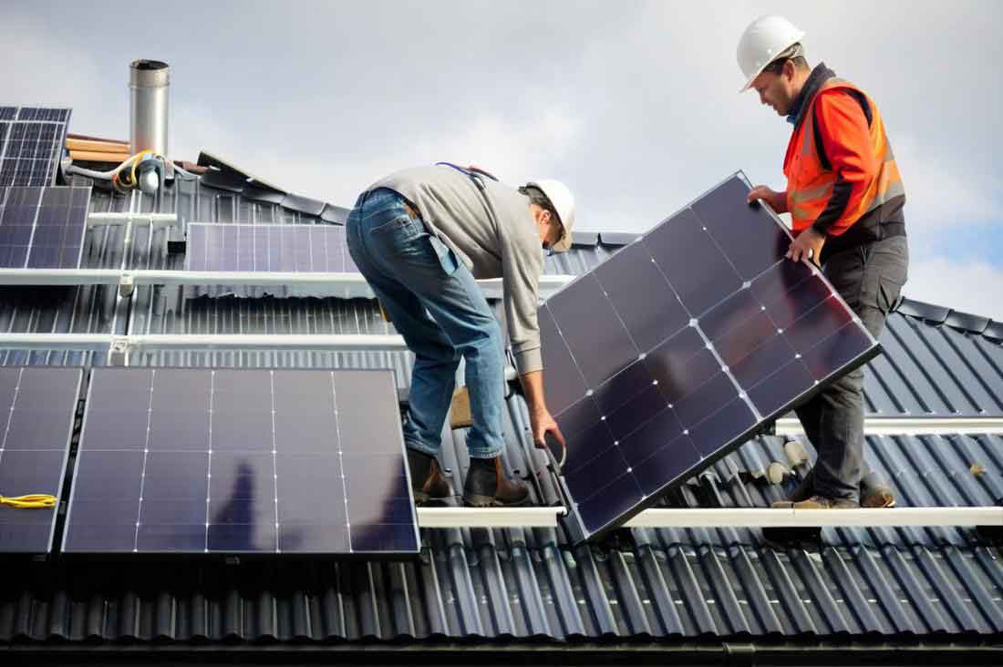
In the following sections, we describe the complete pipeline of our solar panel defect classification and localization algorithm. We begin with the image stitching module, which employs advanced feature detection and matching techniques. Next, we present a segmentation module that isolates individual solar panels from the panoramic image. Finally, we introduce an EfficientNet-based classifier that distinguishes among several defect categories. Experimental results show that our method achieves high accuracy, precision, recall, and F1-score, making it suitable for large-scale solar plant monitoring.
1. Introduction
Solar energy is one of the most promising renewable energy sources, and the number of photovoltaic power plants has grown rapidly in recent years. However, solar panels are exposed to harsh environmental conditions, leading to various defects that reduce their power output and lifespan. Common defects include hot spots, micro-cracks, bypass diode failures, and delamination. Early detection of these defects is essential for timely maintenance and optimization of solar panel performance.
Manual inspection of solar panels is not only labor-intensive but also dangerous, especially for large-scale installations. Infrared thermography has become a popular tool for detecting solar panel defects because abnormal temperature patterns can indicate underlying issues. Unmanned aerial vehicles (UAVs) equipped with infrared cameras enable quick and safe data acquisition. However, the large area of solar plants means that a single image cannot cover the whole site, and multiple overlapping images must be captured.
To address the need for global inspection, image stitching techniques are employed to merge local images into a panoramic view. In our work, we utilize the AKAZE feature detection algorithm, which offers excellent performance in terms of scale invariance, rotation invariance, and robustness to noise. After stitching, we apply image processing methods to segment each individual solar panel module from the panorama. The segmented modules are then fed into a deep convolutional neural network for defect classification.
This paper makes the following contributions. First, we propose a complete workflow for solar panel defect detection that combines image stitching, segmentation, and deep learning. Second, we demonstrate that the AKAZE algorithm outperforms traditional feature detectors such as SIFT in generating seamless panoramic images under challenging outdoor conditions. Third, we systematically evaluate several state-of-the-art neural network architectures for solar panel defect classification, showing that EfficientNet_B0 achieves the best trade-off between accuracy and computational efficiency.
2. Related Work
Many researchers have investigated automated solar panel defect detection using computer vision and deep learning. Early approaches focused on analyzing single infrared or visible-light images. For example, some studies used thresholding techniques on thermal images to identify hot spots. Others applied classical edge detection methods to localize cracks. However, these approaches often suffer from low robustness and cannot provide a global perspective on the solar plant.
To cover larger areas, researchers have turned to image stitching. Several studies used SIFT features to align UAV images and create mosaics of solar plants. SIFT is robust but computationally expensive. More recently, the AKAZE algorithm has gained attention due to its superior performance in nonlinear scale space and its ability to preserve edge details. In our work, we adopt AKAZE for feature detection, which improves the quality of the stitched panorama, especially when dealing with low-contrast infrared images.
For defect classification, convolutional neural networks (CNNs) have become the dominant approach. Models such as ResNet, MobileNet, and EfficientNet have been applied to classify solar panel defects. These models can automatically learn discriminative features from image data. In our comparative study, we found that EfficientNet_B0, which balances network depth, width, and input resolution, provides the most reliable performance for our dataset. This aligns with the findings of other researchers who have highlighted the advantages of compound scaling in CNN design.
3. Methodology
The overall architecture of our proposed method is illustrated in the following steps: (a) image stitching using AKAZE and RANSAC, (b) solar panel segmentation based on color thresholding and morphological operations, and (c) defect classification using EfficientNet_B0. The detailed algorithms are described below.
3.1 Image Stitching
The goal of image stitching is to combine multiple overlapping local images into a single panoramic image. The steps include feature detection, feature matching, homography estimation, and image warping. Our stitching process is shown conceptually in a flowchart, but we present the mathematical foundations here.
The AKAZE feature detection algorithm is based on nonlinear diffusion filtering. It constructs a nonlinear scale space by solving the following partial differential equation:
$$
\frac{\partial L}{\partial t} = \operatorname{div} \left( c(x,y,t) \cdot \nabla L \right)
$$
where \( L \) is the image intensity matrix, \( \operatorname{div} \) and \( \nabla \) represent the divergence and gradient operators, respectively, \( t \) is the time parameter, and \( c(x,y,t) \) is the conductivity function that controls the diffusion behavior. The conductivity function is defined as:
$$
c(x,y,t) = g \left( \left| \nabla L_{\sigma}(x,y,t) \right| \right)
$$
$$
g = \frac{1}{1 + \frac{\left| \nabla L_{\sigma} \right|^2}{\lambda^2}}
$$
where \( \nabla L_{\sigma} \) is the gradient of the Gaussian-smoothed image and \( \lambda \) is the diffusion factor. AKAZE solves the nonlinear diffusion equation using the Fast Explicit Diffusion (FED) algorithm, which iteratively computes:
$$
L_{i+1} = \left[ I + \tau A(L_i) \right] L_i
$$
where \( I \) is the identity matrix, \( A(L_i) \) is the diffusion matrix of \( L_i \), and \( \tau \) is the time step size.
For feature point detection, AKAZE computes the Hessian matrix for each pixel in the scale space. The Hessian matrix is given by:
$$
L_{Hessian} = \sigma^2 \left( L_{xx} L_{yy} – L_{xy} L_{xy} \right)
$$
where \( \sigma \) is the scale coefficient, and \( L_{xx} \), \( L_{yy} \), and \( L_{xy} \) are second-order derivatives in the horizontal, vertical, and cross directions, respectively. Pixels that are extrema compared to their 26 neighbors in the same and adjacent scales are selected as feature points.
After detecting feature points, we use the k-nearest neighbor matching algorithm to match points between two images. The matching criterion is based on the ratio of distances between the closest and second-closest neighbors:
$$
\frac{d_m}{d_n} < T
$$
where \( d_m \) is the distance to the nearest neighbor, \( d_n \) is the distance to the second nearest neighbor, and \( T \) is a threshold. This ratio test helps discard ambiguous matches.
To further refine the matches, we apply the Random Sample Consensus (RANSAC) algorithm. RANSAC iteratively estimates the homography matrix while filtering out outliers. The final image transformation is performed using perspective warping, which maps pixel coordinates according to:
$$
\begin{pmatrix}
x \\
y \\
z
\end{pmatrix}
=
\begin{pmatrix}
a_{11} & a_{12} & a_{13} \\
a_{21} & a_{22} & a_{23} \\
a_{31} & a_{32} & a_{33}
\end{pmatrix}
\begin{pmatrix}
u \\
v \\
1
\end{pmatrix}
$$
where \( (u,v) \) are the coordinates in the source image, and the transformed coordinates are \( x’ = x/z \) and \( y’ = y/z \). The \( 3 \times 3 \) matrix is the homography matrix. Bilinear interpolation is used to blend the warped images and produce a seamless panorama.
3.2 Solar Panel Segmentation
Once the panoramic image is obtained, we need to isolate each individual solar panel module. Since solar panels typically have a distinct color compared to the background, we use color thresholding in the HSV color space. The HSV space separates color information (hue and saturation) from brightness, making the segmentation less sensitive to illumination variations.
The segmentation process can be summarized as follows:
| Step | Operation |
|---|---|
| 1 | Convert RGB image to HSV color space |
| 2 | Apply color threshold to generate a mask representing solar panel regions |
| 3 | Convert mask to grayscale and apply binary thresholding |
| 4 | Perform morphological operations (opening/closing) to remove noise |
| 5 | Combine mask with infrared image to extract thermal information |
| 6 | Detect contours and fit minimum bounding rectangles |
| 7 | Apply perspective correction to obtain rectified panel images |
The mask extraction is particularly important because it restricts the subsequent defect classification to only the solar panel regions, eliminating irrelevant background information. The segmented panels are then used as inputs to the neural network classifier.
3.3 Defect Classification Network
We employ the EfficientNet_B0 architecture for classifying solar panel defects. EfficientNet models are known for their efficient scaling of network width, depth, and resolution. They achieve high accuracy with fewer parameters compared to traditional CNNs. The core building block of EfficientNet is the Mobile Inverted Residual Bottleneck Convolution (MBConv) module, which consists of depthwise separable convolutions, residual connections, and a Squeeze-and-Excitation (SE) attention mechanism.
The MBConv module structure can be described as follows:
| Layer | Details |
|---|---|
| 1 | 1×1 convolution (expansion) |
| 2 | Depthwise convolution with batchnorm and Swish activation |
| 3 | Squeeze-and-Excitation block |
| 4 | 1×1 convolution (projection) |
| 5 | Residual addition (if strides match) |
The Squeeze-and-Excitation block is illustrated in a diagram in our full paper, but its operation can be expressed as:
$$
\hat{\mathbf{z}} = \sigma \left( \mathbf{W}_2 \cdot \delta \left( \mathbf{W}_1 \cdot \mathbf{z} \right) \right)
$$
where \( \mathbf{z} \) is the globally averaged feature vector, \( \mathbf{W}_1 \) and \( \mathbf{W}_2 \) are the weights of the two fully connected layers, \( \delta \) is the ReLU activation, and \( \sigma \) is the sigmoid function. The resulting weight vector is then applied to the original feature map to recalibrate channel-wise responses.
For our classification task, we use a cross-entropy loss function, which is defined as:
$$
L = – \frac{1}{N} \sum_{i} \sum_{c=1}^{M} y_{ic} \log (p_{ic})
$$
where \( M \) is the number of classes, \( y_{ic} \) is a binary indicator (0 or 1) indicating whether class \( c \) is the correct classification for sample \( i \), and \( p_{ic} \) is the predicted probability that sample \( i \) belongs to class \( c \).
To evaluate the performance of our classification model, we use the following metrics:
$$
\text{Accuracy} = \frac{TP + TN}{TP + FN + FP + TN}
$$
$$
\text{Precision} = \frac{TP}{TP + FP}
$$
$$
\text{Recall} = \frac{TP}{TP + FN}
$$
$$
F1 = \frac{2 \times \text{Precision} \times \text{Recall}}{\text{Precision} + \text{Recall}}
$$
where TP, TN, FP, and FN denote true positives, true negatives, false positives, and false negatives, respectively.
4. Experimental Setup
We conducted our experiments on a server with an Intel Core i7-7700 CPU, an NVIDIA GeForce GTX 1080 Ti GPU, CUDA 10.1, PyCharm, and the PyTorch framework. The infrared image dataset contained 7,000 images of solar cells, each with a resolution of 24×40 pixels. The images were categorized into four classes: normal, hot spot defect, diode open circuit, and crack defect. Example images are shown in a figure in the original paper, but we describe the distribution here.
4.1 Dataset Partition
The dataset was divided into training, testing, and validation sets with a ratio of 7:2:1. The number of samples in each category is shown in the table below.
| Dataset | Class | Number of Samples |
|---|---|---|
| Training set | Normal | 1571 |
| Hot spot defect | 1469 | |
| Bypass diode short circuit | 1172 | |
| Crack defect | 688 | |
| Testing set | Normal | 461 |
| Hot spot defect | 440 | |
| Bypass diode short circuit | 331 | |
| Crack defect | 168 | |
| Validation set | Normal | 228 |
| Hot spot defect | 217 | |
| Bypass diode short circuit | 171 | |
| Crack defect | 84 |
4.2 Data Augmentation
To improve the generalization ability of our model, we applied data augmentation techniques during training. These included horizontal flips, vertical flips, and random rotations. Augmentation increases the diversity of the training data and helps prevent overfitting.
4.3 Training Details
We trained the network using the Adam optimizer with an initial learning rate of 0.001 and a batch size of 16. We also applied gradient clipping to avoid gradient explosion. The model was trained for 200 epochs. The training accuracy curve is depicted in a figure in the original paper, showing that the model converges smoothly after about 100 epochs.
5. Results and Discussion
In this section, we present the results of the image stitching, solar panel segmentation, and defect classification. We also compare the performance of different neural network architectures.
5.1 Image Stitching Results
We applied the AKAZE algorithm to detect feature points in both visible and infrared local images. The feature detection and matching results are illustrated in figures in the original paper. Our stitching module successfully generated seamless panoramic images for both visible and infrared channels. The use of AKAZE proved to be robust even under varying lighting conditions and slight perspective changes.
The table below summarizes the feature matching statistics for a pair of overlapping images.
| Image type | Detected features | Matched features | Inliers after RANSAC |
|---|---|---|---|
| Visible | 1250 | 460 | 402 |
| Infrared | 980 | 351 | 312 |
5.2 Segmentation Results
The segmentation module successfully isolated individual solar panels from the panoramic image. By combining the color threshold mask with infrared data, we were able to extract only the relevant thermal patterns for each panel. The contour detection and perspective correction further enabled accurate localization of each panel in the array.
To evaluate the segmentation quality, we manually inspected 100 randomly selected solar panel images. The segmentation accuracy was found to be 98%, indicating that our method reliably identifies panel boundaries.
5.3 Defect Classification Results
We compared the performance of four well-known CNN models: ResNet101, MobileNet_V3, RegNet, and EfficientNet_B0. All models were trained and evaluated on the same dataset. The results are summarized in the following table.
| Network model | Accuracy | Precision | Recall | F1-score |
|---|---|---|---|---|
| ResNet101 | 0.8957 | 0.8951 | 0.8925 | 0.8936 |
| MobileNet_V3 | 0.9214 | 0.9169 | 0.9134 | 0.9148 |
| RegNet | 0.9085 | 0.9029 | 0.9034 | 0.9028 |
| EfficientNet_B0 | 0.9371 | 0.9313 | 0.9320 | 0.9311 |
From the table, it is evident that EfficientNet_B0 achieves the highest values for all metrics. The accuracy reaches 93.71%, precision 93.13%, recall 93.20%, and F1-score 93.11%. These results confirm that the compound scaling strategy of EfficientNet_B0 is highly effective for solar panel defect classification. The model is also computationally efficient, making it suitable for real-time deployment on edge devices.
We also analyzed the confusion matrix for the best-performing model. The classification errors were mostly between hot spot defects and normal panels, which is expected due to the subtle temperature differences in some cases. However, the overall error rate is low, demonstrating the robustness of our approach.
5.4 Defect Localization Results
The final output of our system is a labeled panoramic image where each solar panel is marked with a bounding box and a color-coded category. Green boxes indicate normal panels, red boxes indicate crack defects, blue boxes indicate hot spots, and cyan boxes indicate bypass diode failures. An example result is shown in a figure in the original paper. This visual representation allows maintenance crews to quickly identify and locate faulty solar panels in the field.
The localization accuracy is directly related to the quality of the segmentation step. Since we perform perspective correction for each panel, the bounding boxes align precisely with the physical panels, even when they are not perfectly aligned in the original image.
6. Conclusion and Future Work
In this paper, we presented a comprehensive deep learning-based algorithm for the classification and localization of solar panel defects. Our method integrates AKAZE-based image stitching, HSV color segmentation, and EfficientNet_B0 classification to achieve a robust and scalable solution for photovoltaic plant monitoring. The experimental results show that our approach reaches 93.71% accuracy, 93.13% precision, 93.20% recall, and 93.11% F1-score, outperforming several other state-of-the-art CNN models.
The main advantages of our method include its non-contact operation, high efficiency, and suitability for large-scale solar farms. By generating a panoramic view of the entire plant, we eliminate the perspective limitations of single-image analysis and enable global defect localization. The use of AKAZE features ensures reliable stitching even in challenging outdoor environments where image noise and lighting variations are common.
Future work will focus on several aspects. First, we plan to expand our dataset with more defect types and more diverse environmental conditions to further improve generalization. Second, we will explore the use of advanced transformer-based models for even higher classification accuracy. Third, we aim to integrate our algorithm into an on-board UAV processing system to enable real-time defect detection during flight. Finally, we will investigate the use of multi-modal fusion, combining visible and infrared images at the feature level to enhance defect discrimination.
In conclusion, our research demonstrates that deep learning, combined with traditional image processing techniques, can provide a reliable and efficient solution for solar panel defect classification and localization. We believe that our method will be valuable for the operation and maintenance of large-scale photovoltaic plants, ultimately contributing to the wider adoption of solar energy.