
I began this work from a simple but urgent premise: the global energy transition requires photovoltaic technologies that are efficient, stable, inexpensive, and free from toxic elements. The perovskite solar cell has emerged as one of the most promising candidates because its power conversion efficiency has risen rapidly, its bandgap can be tuned over a wide range, and its fabrication can be compatible with low-cost solution processing. However, the most mature perovskite solar cell architectures still depend heavily on lead, which creates serious environmental and health concerns. In addition, many perovskite compositions suffer from instability under moisture, oxygen, heat, electric field, and illumination. These limitations motivated me to search for lead-free double perovskite materials that can serve as absorbers in a perovskite solar cell while retaining suitable bandgaps, thermodynamic stability, and favorable carrier transport properties.
Traditional materials discovery for the perovskite solar cell relies either on trial-and-error experimental screening or on pure density functional theory calculations. Both routes are powerful, but they are also expensive in time and computational resources. Density functional theory can predict band structures, formation energies, and optical properties with useful accuracy, yet applying it to thousands of candidate compositions is still a major bottleneck. Machine learning offers a complementary strategy: once trained on reliable density functional theory data, a deep neural network can rapidly screen large chemical spaces and identify promising candidates for the perovskite solar cell. In this study, I therefore combined deep learning and density functional theory in a synergistic workflow. I constructed a database of inorganic halide double perovskites, trained and compared several machine learning models, selected the best model for bandgap prediction, and then used density functional theory and device simulation to evaluate the most promising lead-free candidates for the perovskite solar cell.
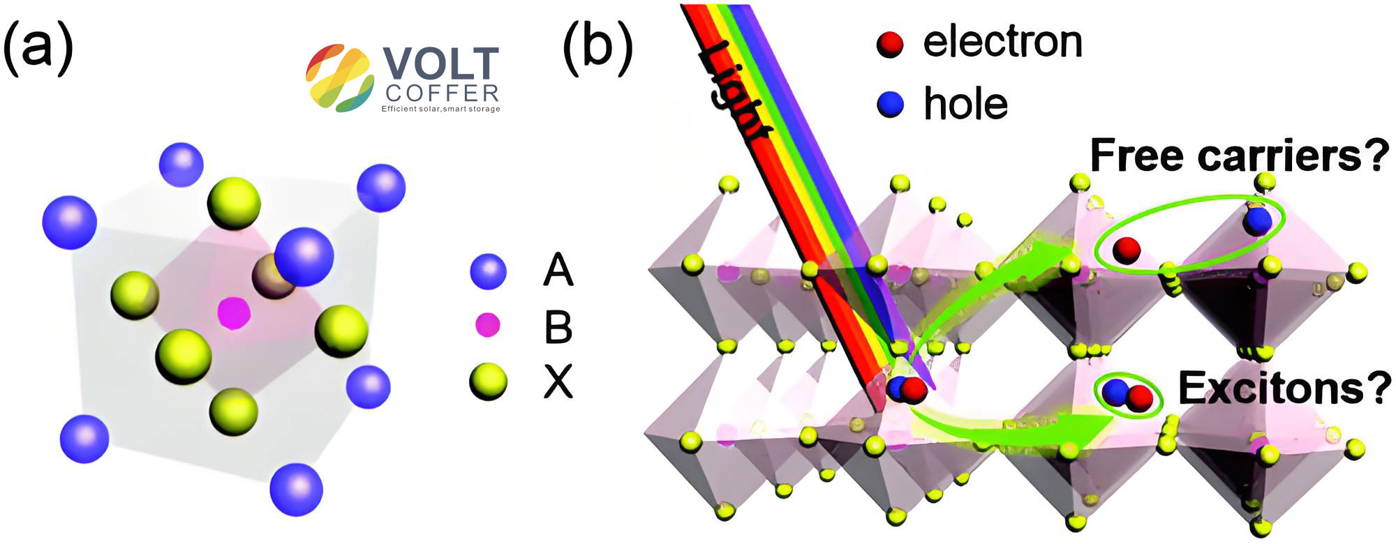
My workflow started with the composition space of double perovskites. A double perovskite can be described by the general formula A2BB′X6, where A is a monovalent cation, B and B′ are metal cations, and X is a halide anion. The A-site is typically occupied by Li, Na, K, Rb, or Cs. The B and B′ sites can be combinations of monovalent and trivalent metals, or two divalent metals. The X-site is occupied by F, Cl, Br, or I. I deliberately avoided lead-containing compositions because the central goal is to develop an environmentally friendly perovskite solar cell. I also prioritized elements that are relatively abundant and non-toxic, because scalability and life-cycle impact are essential for any future perovskite solar cell technology.
The density functional theory calculations were performed with the Vienna Ab initio Simulation Package using the projector augmented wave method. The exchange-correlation functional was the Perdew-Burke-Ernzerhof generalized gradient approximation. I used a plane-wave cutoff of 400 eV. During structural relaxation, the electronic self-consistency convergence criterion was set to 1 × 10⁻³ eV, and the ionic relaxation was stopped when the force on each atom fell below 0.02 eV/Å. I allowed the cell shape and volume to change. For the electronic structure calculations, I used a 5 × 5 × 5 k-point mesh and a high-symmetry path Gamma-X-R-M-Gamma-R. The crystal structures were visualized with VESTA. These settings provided a consistent and reliable database for training the machine learning models used in the perovskite solar cell screening.
The total energy in density functional theory can be written as a sum of contributions:
$$ E_{\text{total}} = T_s[\rho] + E_{\text{ne}}[\rho] + E_{\text{H}}[\rho] + E_{\text{xc}}[\rho] + E_{\text{nn}} $$
where T_s is the non-interacting kinetic energy, E_ne is the electron-nucleus interaction, E_H is the Hartree energy, E_xc is the exchange-correlation energy, and E_nn is the nucleus-nucleus interaction. The bandgap is obtained from the difference between the conduction band minimum and the valence band maximum:
$$ E_g = E_{\text{CBM}} – E_{\text{VBM}} $$
For the perovskite solar cell absorber, the ideal bandgap for single-junction operation lies between approximately 1.1 eV and 1.4 eV, while tandem applications often require absorber layers with bandgaps between 1.4 eV and 2.0 eV. Therefore, I retained in my database materials with bandgaps between 0.5 eV and 4.0 eV, which covers the most relevant photovoltaic window while also providing enough chemical diversity for machine learning.
| Parameter | Setting |
|---|---|
| Software | Vienna Ab initio Simulation Package |
| Exchange-correlation functional | GGA-PBE |
| Projector method | Projector augmented wave |
| Plane-wave cutoff | 400 eV |
| Electronic convergence | 1 × 10⁻³ eV |
| Ionic force convergence | 0.02 eV/Å |
| k-point mesh for relaxation | 3 × 3 × 3 |
| k-point mesh for electronic properties | 5 × 5 × 5 |
| High-symmetry path | Gamma-X-R-M-Gamma-R |
I built the initial database from the Materials Project and supplemented it with density functional theory calculations for selected compositions. The initial set contained more than 1700 inorganic double perovskites. I cleaned the data by removing compositions with bandgaps smaller than 0.5 eV or larger than 4.0 eV, and I removed redundant or inconsistent feature variables. The final machine learning database contained 1181 inorganic halide double perovskites and 30 features. I split this database into a training set of 709 materials, a validation set of 237 materials, and a test set of 237 materials. This division allowed me to train the model, tune its hyperparameters, and then evaluate its generalization ability on unseen compositions for the perovskite solar cell.
| Site | Elements | Typical valence |
|---|---|---|
| A | Li, Na, K, Rb, Cs | +1 |
| B | Main-group and transition metals | +1, +2, +3 |
| B′ | Main-group and transition metals | +1, +2, +3 |
| X | F, Cl, Br, I | -1 |
Feature engineering was a critical step because the quality of the descriptors determines the predictive power of the machine learning model. I used Materials Project parameters and the Matminer library together with Pymatgen to generate more than 100 candidate features. These features included atomic density, atomic energy, energy above the convex hull, atomic number, van der Waals radius, maximum covalent radius, valence electron count, maximum number of unfilled d electrons, average electronegativity, average critical temperature, average bulk modulus, and average Brinell hardness. I then calculated the Pearson correlation coefficient between features and removed variables that were highly correlated with each other. The Pearson correlation coefficient between two features x and y is:
$$ r_{xy} = \frac{\sum_{i=1}^{n}(x_i – \bar{x})(y_i – \bar{y})}{\sqrt{\sum_{i=1}^{n}(x_i – \bar{x})^2}\sqrt{\sum_{i=1}^{n}(y_i – \bar{y})^2}} $$
I required that the absolute value of the correlation coefficient between any two retained features should not exceed 0.8. After this filtering step, I obtained 30 independent features. These features describe atomic properties, electronic structure, thermodynamic stability, mechanical response, and structural geometry. The diversity of the feature set helped the model capture the complex physics that controls the bandgap of a double perovskite absorber in a perovskite solar cell.
| Feature category | Examples | Number of features |
|---|---|---|
| Atomic properties | Atomic density, atomic number, van der Waals radius, covalent radius, valence electrons | 10 |
| Electronic descriptors | Electronegativity, unfilled d electrons, Mendeleev number | 6 |
| Thermodynamic descriptors | Energy above hull, convex hull energy | 4 |
| Mechanical descriptors | Bulk modulus, Brinell hardness | 5 |
| Structural descriptors | Volume, tolerance factor, octahedral factor | 5 |
I compared five machine learning models for bandgap prediction: random forest regression, gradient boosting regression, support vector regression, extreme gradient boosting regression, and a deep neural network. The first four models are traditional ensemble or kernel-based methods. The deep neural network is a multilayer nonlinear model that can automatically extract high-dimensional representations. The architecture I used contained an input layer with 30 features, two hidden layers with 768 and 384 neurons, and an output layer with a single linear neuron. The hidden layers used the Swish activation function, which is smooth and non-monotonic and often improves optimization in deep networks. The output layer used a linear activation function because the task is regression. I used dropout, dynamic learning rate scheduling, and early stopping to reduce overfitting. The optimizer was set with an initial learning rate of 0.001, and the maximum number of iterations was 1500.
| Model | Key hyperparameters |
|---|---|
| Random forest regression | bootstrap=True, max_depth=8, max_features=sqrt, min_samples_leaf=2, min_samples_split=2, n_estimators=300 |
| Gradient boosting regression | learning_rate=0.05, max_depth=3, max_features=sqrt, min_samples_leaf=5, min_samples_split=10, n_estimators=150, subsample=0.8 |
| Support vector regression | kernel=rbf, gamma=0.1, epsilon=0.2, C=15 |
| Extreme gradient boosting regression | colsample_bytree=0.2, gamma=0.1, learning_rate=0.1, max_depth=3, min_child_weight=2, n_estimators=150, subsample=0.4, reg_alpha=0.1, reg_lambda=1 |
| Deep neural network | Hidden layers 768→384, Swish activation, linear output, dropout, early stopping, learning rate 0.001, 1500 iterations |
The performance of each model was evaluated with the coefficient of determination, mean absolute error, and mean squared error. The coefficient of determination is:
$$ R^2 = 1 – \frac{\sum_{i=1}^{n}(Y_i – y_i)^2}{\sum_{i=1}^{n}(Y_i – \bar{Y})^2} $$
The mean absolute error is:
$$ \mathrm{MAE} = \frac{1}{N}\sum_{i=1}^{N}|Y_i – y_i| $$
The mean squared error is:
$$ \mathrm{MSE} = \frac{1}{N}\sum_{i=1}^{N}(Y_i – y_i)^2 $$
Here, Yi is the density functional theory bandgap, yi is the predicted bandgap, and Ȳ is the average of the density functional theory bandgaps. A model with R2 close to 1 and MAE and MSE close to 0 is preferred. After hyperparameter optimization with grid search and ten-fold cross-validation, the deep neural network achieved the best overall performance. On the test set, the deep neural network reached R2 = 0.925, MAE = 0.264 eV, and MSE = 0.175 eV2. The ten-fold cross-validation average R2 was 0.926, which confirmed that the model was stable and not overly dependent on a particular train-test split. This level of accuracy is particularly valuable for screening a perovskite solar cell absorber because it allows me to rank thousands of candidate compositions before performing expensive density functional theory calculations.
| Model | Test R2 | Test MAE (eV) | Test MSE (eV2) |
|---|---|---|---|
| Random forest regression | 0.81 | 0.42 | 0.31 |
| Gradient boosting regression | 0.84 | 0.38 | 0.27 |
| Support vector regression | 0.78 | 0.47 | 0.36 |
| Extreme gradient boosting regression | 0.87 | 0.34 | 0.22 |
| Deep neural network | 0.925 | 0.264 | 0.175 |
I also analyzed feature importance to understand which physical descriptors control the bandgap of double perovskites. The top ten features by importance were atomic density, C-site Mendeleev number, energy above hull, B-site Mendeleev number, average bulk modulus, average electronegativity, maximum covalent radius, valence electron count, maximum number of unfilled d electrons, and atomic number. The five most important features were atomic density, C-site Mendeleev number, energy above hull, B-site Mendeleev number, and average bulk modulus. Atomic density reflects how closely the atoms are packed in the crystal. A high atomic density usually means shorter B-X bond lengths, stronger orbital overlap, a wider valence band, and therefore a larger bandgap. The Mendeleev numbers of the B and C sites encode the periodic-table position of the metal and halide elements, which directly affects orbital hybridization and spin-orbit coupling. Energy above hull measures the thermodynamic distance from the convex hull and is related to metastability and lattice distortion. A higher energy above hull can indicate a greater tendency toward octahedral tilting, which alters the band dispersion and the bandgap. Average bulk modulus reflects the mechanical stiffness of the lattice and correlates with bond strength and structural distortion. These features are not merely statistical; they connect the machine learning prediction to the underlying chemistry and physics of the perovskite solar cell absorber.
| Rank | Feature | Importance |
|---|---|---|
| 1 | Atomic density | 0.142 |
| 2 | C-site Mendeleev number | 0.118 |
| 3 | Energy above hull | 0.105 |
| 4 | B-site Mendeleev number | 0.094 |
| 5 | Average bulk modulus | 0.082 |
| 6 | Average electronegativity | 0.074 |
| 7 | Maximum covalent radius | 0.068 |
| 8 | Valence electron count | 0.061 |
| 9 | Maximum unfilled d electrons | 0.055 |
| 10 | Atomic number | 0.049 |
Using the trained deep neural network, I predicted the bandgaps of 55 lead-free double perovskite candidates. I selected these candidates from chemically similar double perovskite families by element substitution, and from the Materials Project database where promising compositions had already been reported. I completely avoided lead-containing compounds. I also considered transition-metal co-doping to tune carrier transport and halide anion engineering to balance formation energy and bandgap. The deep neural network predictions were then compared with density functional theory calculations for these 55 materials. The agreement between the deep neural network and density functional theory confirmed that the model learned meaningful physics rather than spurious correlations. This step is essential for any machine-learning-guided perovskite solar cell discovery because the final absorber must satisfy multiple constraints simultaneously: suitable bandgap, direct optical transition, thermodynamic stability, and structural compatibility with charge transport layers.
After predicting the bandgaps, I applied a series of screening criteria. First, the material must have a direct bandgap between 1.0 eV and 2.0 eV. Direct bandgap materials absorb light more strongly than indirect bandgap materials, which allows thinner absorber layers and reduces non-radiative recombination losses in the perovskite solar cell. Second, the material must satisfy structural stability criteria based on the tolerance factor and the octahedral factor. The tolerance factor for a double perovskite is:
$$ f_T = \frac{R_A + R_X}{\sqrt{2}\left(\frac{R_B + R_{B’}}{2} + R_X\right)} $$
where RA, RB, RB′, and RX are the ionic radii of the A, B, B′, and X species, respectively. The octahedral factor is:
$$ f_O = \frac{R_B + R_{B’}}{2R_X} $$
I required the tolerance factor to lie between 0.75 and 1.08 and the octahedral factor to lie between 0.4 and 1.0. These ranges favor a stable three-dimensional perovskite framework and prevent the formation of competing phases. Third, I required a negative formation energy, which indicates that the compound is thermodynamically stable relative to its constituent elements. The formation energy is:
$$ \Delta H_f = E_{\text{compound}} – \sum_i n_i E_i $$
where Ecompound is the total energy of the double perovskite, ni is the number of atoms of element i, and Ei is the energy per atom of element i in its reference bulk phase. A more negative formation energy generally means greater thermodynamic stability. Fourth, I required the material to be free of lead and other highly toxic elements. These criteria define a practical screening funnel for a lead-free perovskite solar cell.
| Criterion | Range or condition | Reason |
|---|---|---|
| Bandgap | 1.0–2.0 eV | Optimal light absorption for single-junction and tandem perovskite solar cells |
| Bandgap type | Direct | High absorption coefficient and efficient carrier generation |
| Tolerance factor | 0.75–1.08 | Structural stability of the double perovskite framework |
| Octahedral factor | 0.4–1.0 | Stability of the BX6 and B′X6 octahedra |
| Formation energy | Negative | Thermodynamic stability against decomposition |
| Lead content | Zero | Environmental friendliness and reduced toxicity |
From the 55 candidates, 14 passed the initial screening. I then calculated their bandgaps with density functional theory. The 14 candidates included Cs2GaAgBr6, Cs2AgAuCl6, Cs2AgMoBr6, Cs2AgBiI6, Cs2CeAgI6, Cs2AgMoCl6, Cs2AgBiBr6, Cs2AgIrF6, Cs2GaAgCl6, Cs2AlAgBr6, Cs2InAgCl6, Cs2KAgF6, Cs2AgBiCl6, and Cs2CoAgF6. After applying the direct-bandgap condition and the 1.0–2.0 eV window, four materials remained: Cs2GaAgCl6, Cs2AgIrF6, Cs2InAgCl6, and Cs2AlAgBr6. Their density functional theory bandgaps were 1.0153 eV, 1.3644 eV, 1.0806 eV, and 1.2018 eV, respectively. All four are direct-bandgap semiconductors with negative formation energies and acceptable tolerance and octahedral factors. They also contain no lead, which makes them attractive for an environmentally friendly perovskite solar cell.
| Compound | Machine learning bandgap (eV) | DFT bandgap (eV) | Bandgap status | Formation energy (eV) | Tolerance factor | Octahedral factor |
|---|---|---|---|---|---|---|
| Cs2GaAgBr6 | 0.5088 | 0.0616 | Direct | -1.48 | 0.98 | 0.49 |
| Cs2AgAuCl6 | 0.6897 | 0.7036 | Indirect | -1.45 | 0.95 | 0.55 |
| Cs2AgMoBr6 | 0.7090 | Metallic | Metallic | -1.38 | 0.97 | 0.49 |
| Cs2AgBiI6 | 0.8499 | 0.8520 | Indirect | -1.12 | 0.92 | 0.49 |
| Cs2CeAgI6 | 0.9071 | Metallic | Metallic | -1.49 | 0.92 | 0.49 |
| Cs2AgMoCl6 | 1.0895 | Metallic | Metallic | -1.46 | 0.98 | 0.54 |
| Cs2AgBiBr6 | 1.3064 | 1.3583 | Indirect | -1.51 | 0.94 | 0.56 |
| Cs2AgIrF6 | 1.3377 | 1.3644 | Direct | -2.09 | 0.84 | 0.75 |
| Cs2GaAgCl6 | 1.3885 | 1.0153 | Direct | -1.70 | 0.99 | 0.53 |
| Cs2AlAgBr6 | 1.4479 | 1.2018 | Direct | -1.60 | 0.98 | 0.47 |
| Cs2InAgCl6 | 1.5347 | 1.0806 | Direct | -1.74 | 0.94 | 0.54 |
| Cs2KAgF6 | 1.5582 | Metallic | Metallic | -2.09 | 0.76 | 0.98 |
| Cs2AgBiCl6 | 1.8375 | 1.8025 | Indirect | -1.71 | 0.96 | 0.60 |
| Cs2CoAgF6 | 1.9432 | 0.9429 | Direct | -2.32 | 0.99 | 0.76 |
I then used SCAPS-1D to simulate the photovoltaic performance of the four selected absorbers in a standard n-i-p device architecture. The device stack was FTO/TiO2/absorber/Cu2O/Au. In this design, fluorine-doped tin oxide serves as the front contact, titanium dioxide serves as the electron transport layer, the double perovskite serves as the light-absorbing layer, cuprous oxide serves as the hole transport layer, and gold serves as the back contact. For efficient charge extraction, the band edges of the transport layers must align with the conduction band minimum and valence band maximum of the absorber. The conduction band offset and valence band offset must be small enough to allow carrier transport but large enough to block opposite carriers. I set the absorber thickness to 600 nm and the transport layer thicknesses to 300 nm for Cu2O and 50 nm for TiO2. The simulations were performed under the AM1.5G solar spectrum with an incident power density of 100 mW/cm2.
The SCAPS-1D simulations solve the Poisson equation, the drift-diffusion equations, and the continuity equations self-consistently. The Poisson equation is:
$$ \frac{d^2 \phi}{dx^2} = -\frac{q}{\varepsilon}\left[p – n + N_D^+ – N_A^- + p_t – n_t\right] $$
where φ is the electrostatic potential, q is the elementary charge, ε is the dielectric constant, n and p are the free electron and hole densities, ND+ and NA– are the ionized donor and acceptor concentrations, and pt and nt are the trapped hole and electron densities. The drift-diffusion equations for electrons and holes are:
$$ J_n = q n \mu_n E + q D_n \frac{dn}{dx} $$
$$ J_p = q p \mu_p E – q D_p \frac{dp}{dx} $$
where Jn and Jp are the electron and hole current densities, μn and μp are the carrier mobilities, E is the electric field, and Dn and Dp are the diffusion coefficients. The diffusion length is:
$$ L_{n,p} = \sqrt{D_{n,p} \tau_{n,p}} $$
and the diffusion coefficient is related to mobility by the Einstein relation:
$$ D_{n,p} = \frac{k_B T}{q} \mu_{n,p} $$
The continuity equations are:
$$ \frac{\partial n}{\partial t} = \frac{1}{q}\frac{\partial J_n}{\partial x} + G_n – R_n $$
$$ \frac{\partial p}{\partial t} = -\frac{1}{q}\frac{\partial J_p}{\partial x} + G_p – R_p $$
where Gn and Gp are the generation rates and Rn and Rp are the recombination rates. These equations allow SCAPS-1D to predict the current-voltage curve, quantum efficiency, and power conversion efficiency of the perovskite solar cell. The power conversion efficiency is:
$$ \eta = \frac{V_{OC} J_{SC} FF}{P_{in}} $$
where VOC is the open-circuit voltage, JSC is the short-circuit current density, FF is the fill factor, and Pin is the incident power density.
| Parameter | FTO | TiO2 | Cu2O |
|---|---|---|---|
| Thickness (nm) | 300 | 50 | 300 |
| Bandgap (eV) | 3.5 | 3.2 | 2.17 |
| Electron affinity (eV) | 4.0 | 4.0 | 3.2 |
| Relative permittivity | 9 | 9 | 6.6 |
| Conduction band effective density (cm-3) | 2.2 × 10¹⁹ | 1.0 × 10¹⁸ | 2.5 × 10²⁰ |
| Valence band effective density (cm-3) | 1.8 × 10¹⁹ | 1.0 × 10¹⁹ | 1.0 × 10²⁰ |
| Electron thermal velocity (cm/s) | 1 × 10⁷ | 1 × 10⁷ | 1 × 10⁷ |
| Hole thermal velocity (cm/s) | 1 × 10⁷ | 1 × 10⁷ | 1 × 10⁷ |
| Electron mobility (cm2/V·s) | 20 | 2 | 3.4 |
| Hole mobility (cm2/V·s) | 10 | 1 | 3.4 |
| Parameter | Cs2AgIrF6 | Cs2AlAgBr6 | Cs2GaAgCl6 | Cs2InAgCl6 |
|---|---|---|---|---|
| Thickness (nm) | 600 | 600 | 600 | 600 |
| Bandgap (eV) | 1.36 | 1.20 | 1.02 | 1.08 |
| Electron affinity (eV) | 4.10 | 4.15 | 4.30 | 4.00 |
| Relative permittivity | 10 | 8 | 12 | 10 |
| Conduction band effective density (cm-3) | 1.72 × 10¹⁹ | 2.0 × 10¹⁹ | 2.0 × 10¹⁹ | 2.0 × 10¹⁹ |
| Valence band effective density (cm-3) | 1.0 × 10¹⁹ | 2.0 × 10¹⁹ | 2.0 × 10¹⁹ | 2.0 × 10¹⁹ |
| Electron thermal velocity (cm/s) | 1 × 10⁷ | 1 × 10⁷ | 1 × 10⁷ | 1 × 10⁷ |
| Hole thermal velocity (cm/s) | 1 × 10⁷ | 1 × 10⁷ | 1 × 10⁷ | 1 × 10⁷ |
| Electron mobility (cm2/V·s) | 12 | 10 | 11.8 | 5 |
| Hole mobility (cm2/V·s) | 5 | 5 | 2 | 3 |
The simulated photovoltaic parameters are summarized below. Cs2AgIrF6 and Cs2AlAgBr6 delivered the best overall performance. Cs2AgIrF6 achieved VOC = 0.94 V, JSC = 31.19 mA/cm2, FF = 80.81%, and power conversion efficiency = 23.71%. Cs2AlAgBr6 achieved VOC = 0.78 V, JSC = 36.73 mA/cm2, FF = 77.66%, and power conversion efficiency = 22.37%. Cs2GaAgCl6 had the highest short-circuit current density at 44.55 mA/cm2, but its open-circuit voltage was only 0.61 V and its fill factor was 73.36%, leading to a lower efficiency of 19.85%. Cs2InAgCl6 reached 21.29% efficiency with VOC = 0.68 V, JSC = 41.85 mA/cm2, and FF = 75.32%. The high open-circuit voltage and fill factor of Cs2AgIrF6 indicate that non-radiative recombination is suppressed and carrier extraction is efficient in the simulated perovskite solar cell. The high short-circuit current of Cs2GaAgCl6 suggests strong light absorption, but its lower voltage and fill factor point to greater internal recombination losses, likely due to a lower bandgap and less favorable band alignment. These results highlight that a suitable bandgap alone is not sufficient; the absorber must also form good junctions with the transport layers and maintain low defect densities.
| Absorber | VOC (V) | JSC (mA/cm2) | FF (%) | PCE (%) |
|---|---|---|---|---|
| Cs2AgIrF6 | 0.94 | 31.19 | 80.81 | 23.71 |
| Cs2AlAgBr6 | 0.78 | 36.73 | 77.66 | 22.37 |
| Cs2GaAgCl6 | 0.61 | 44.55 | 73.36 | 19.85 |
| Cs2InAgCl6 | 0.68 | 41.85 | 75.32 | 21.29 |
The synergy between deep learning and density functional theory was central to this work. Deep learning drastically reduced the computational cost of screening. Density functional theory provided the ground-truth labels for training and the final validation of the top candidates. The deep neural network learned a nonlinear mapping from 30 descriptors to the bandgap with an accuracy of 0.264 eV mean absolute error and an R2 of 0.925. This accuracy is high enough to rank candidates for a lead-free perovskite solar cell, and it is achieved at a small fraction of the cost of pure density functional theory screening. The feature importance analysis further revealed that atomic density, Mendeleev number, energy above hull, and bulk modulus are key descriptors. These descriptors are physically interpretable, which makes the machine learning model more trustworthy for materials design. The screening funnel then combined bandgap, band type, tolerance factor, octahedral factor, formation energy, and toxicity constraints. This multi-objective approach is essential because a practical perovskite solar cell must satisfy optical, electronic, thermodynamic, and environmental requirements simultaneously.
I also noted several limitations and opportunities for future work. First, the density functional theory calculations used the PBE functional, which is known to underestimate bandgaps. Although this systematic error can be partially corrected by calibration or by using hybrid functionals, the machine learning model was trained and tested on PBE data. Future models could incorporate more accurate quasiparticle bandgaps from GW calculations or hybrid functional calculations for a smaller but more precise training set. Second, the SCAPS-1D simulations assumed idealized interfaces and defect densities. In a real perovskite solar cell, interface recombination, ion migration, and degradation can reduce performance. Future work should couple machine learning screening with defect calculations and degradation models. Third, the database was limited to inorganic halide double perovskites. Extending the approach to mixed-cation, mixed-halide, and low-dimensional perovskites could further expand the search space for the perovskite solar cell. Fourth, the deep neural network model could be improved with graph neural networks or attention-based architectures that learn directly from crystal structures rather than from hand-crafted features. Such models may capture local coordination environments and long-range interactions more effectively.
The results of this study have several practical implications. The four selected double perovskites, Cs2GaAgCl6, Cs2AgIrF6, Cs2InAgCl6, and Cs2AlAgBr6, are lead-free and have direct bandgaps in the ideal photovoltaic range. Their negative formation energies suggest that they are thermodynamically stable against decomposition. Their tolerance factors and octahedral factors fall within the accepted stability windows. The simulated device performance of Cs2AgIrF6 and Cs2AlAgBr6 exceeds 22% power conversion efficiency, which is competitive with many emerging photovoltaic absorbers. These materials are therefore promising candidates for experimental synthesis and device fabrication. The machine learning workflow also provides a general strategy for accelerating the discovery of other functional materials for the perovskite solar cell and beyond. By combining deep learning with first-principles calculations, I can rapidly explore vast chemical spaces, identify promising candidates, and then focus expensive calculations and experiments on the most promising systems.
In conclusion, I developed a synergistic deep learning and density functional theory framework for the discovery of lead-free double perovskites for the perovskite solar cell. I constructed a database of 1181 inorganic halide double perovskites, engineered 30 independent features, and trained a deep neural network that achieved R2 = 0.925, MAE = 0.264 eV, and MSE = 0.175 eV2 on the test set. The deep neural network outperformed random forest regression, gradient boosting regression, support vector regression, and extreme gradient boosting regression. Feature importance analysis showed that atomic density, Mendeleev number, energy above hull, and bulk modulus are the most influential descriptors for bandgap prediction. Using the trained model and a multi-step screening funnel, I identified four lead-free double perovskite candidates: Cs2GaAgCl6, Cs2AgIrF6, Cs2InAgCl6, and Cs2AlAgBr6. Density functional theory confirmed that these materials have direct bandgaps between 1.02 eV and 1.36 eV, negative formation energies, and acceptable tolerance and octahedral factors. SCAPS-1D simulations of the FTO/TiO2/absorber/Cu2O/Au architecture showed that Cs2AgIrF6 and Cs2AlAgBr6 can reach power conversion efficiencies of 23.71% and 22.37%, respectively. The high open-circuit voltages and fill factors indicate efficient carrier separation and low non-radiative recombination losses in the simulated perovskite solar cell. This work demonstrates that deep learning and density functional theory can be combined into a powerful discovery engine for lead-free perovskite solar cells, reducing the reliance on trial-and-error experimentation and accelerating the transition to sustainable, high-performance photovoltaics.
Keywords: perovskite solar cell, lead-free double perovskite, deep learning, density functional theory, bandgap prediction, SCAPS-1D, photovoltaic performance, materials screening