
I have conducted a comprehensive investigation into the remaining useful life (RUL) prediction of lithium-ion cells because the health state of a lithium-ion cell directly determines the safety, reliability, and total cost of ownership of energy storage systems, portable electronics, and electric vehicles. The degradation of a lithium-ion cell is governed by complex electrochemical processes that are coupled with temperature, charge-discharge rate, and operating environment. These factors make accurate lifetime prediction a difficult task. In my work, I propose a data-driven prediction system that uses a long short-term memory (LSTM) network to forecast the remaining useful life of a lithium-ion cell. The system first preprocesses raw capacity data, then applies an autoregressive method to handle the time series, then divides the dataset with a sliding window, and finally trains an LSTM model. I evaluate the system on the CALCE dataset. Compared with a convolutional neural network (CNN) model, my LSTM model improves relative error (RE), mean absolute error (MAE), and root mean square error (RMSE) by approximately 16.30%, 42.08%, and 30.36%, respectively. This system largely solves the problem of inaccurate remaining useful life prediction for lithium-ion cells and can provide technical support for rationally arranging charging plans and improving energy utilization efficiency.
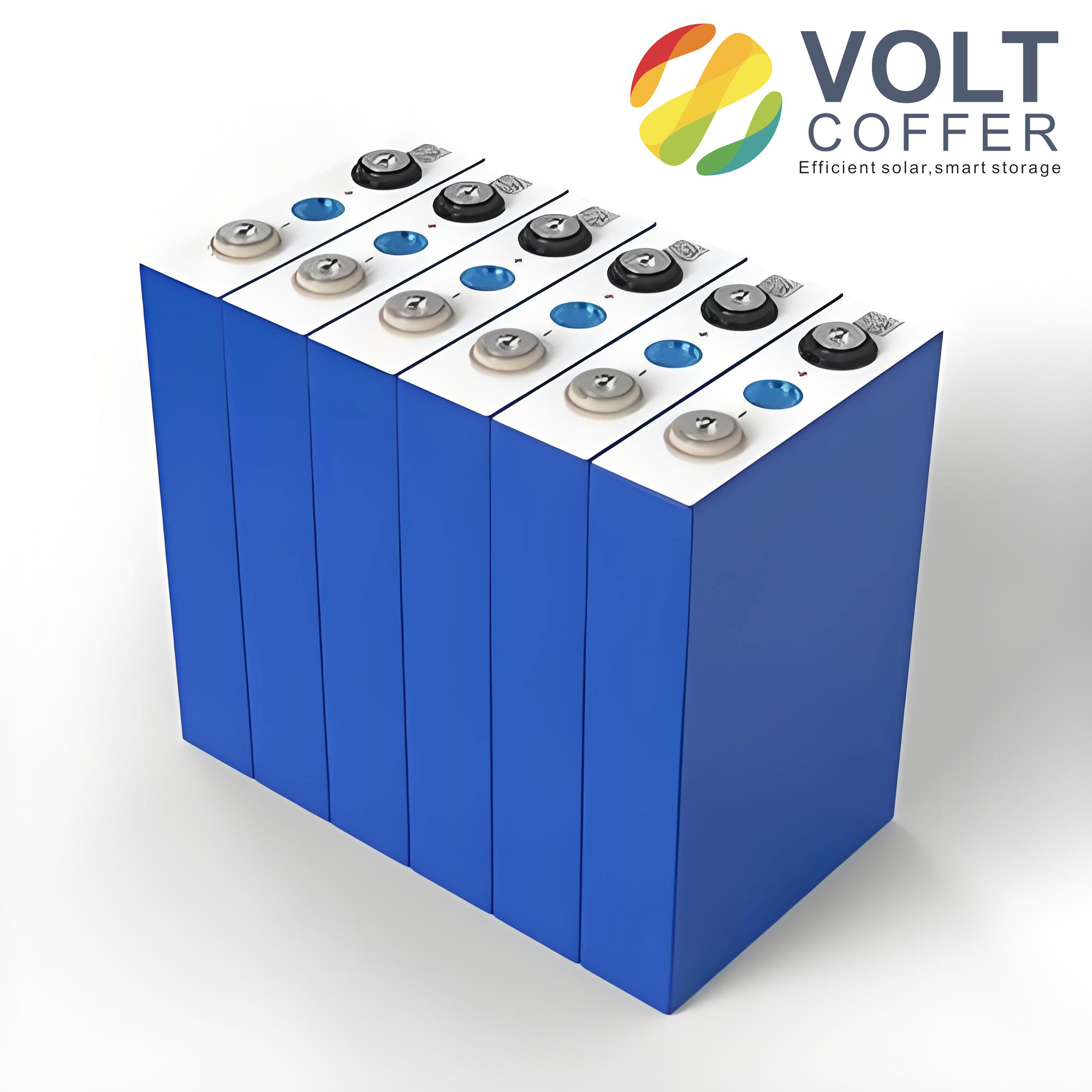
In my view, the lithium-ion cell is the core energy carrier of modern green energy systems. Its state of health (SOH) and remaining useful life are critical for safe operation. The RUL of a lithium-ion cell is usually defined as the number of charge-discharge cycles remaining before the capacity fades to a predefined end-of-life threshold, such as 70% or 80% of the rated capacity. I denote the capacity at cycle \( t \) as \( C_t \). The end-of-life threshold is \( C_{EOL} \). Then the RUL at cycle \( t \) is:
$$ RUL_t = \min \{ k \in \mathbb{N} : C_{t+k} \leq C_{EOL} \} $$
Because the internal chemical reactions of a lithium-ion cell are complex, model-driven methods based on electrochemical mechanisms or equivalent circuits often require tedious modeling and parameter identification. They also have poor universality under complex practical conditions. Data-driven methods, in contrast, mine degradation patterns from full-lifecycle monitoring data without deeply exploring the internal electrochemical mechanism. They are convenient and have strong generalization ability. Therefore, data-driven methods have become a mainstream research direction for lithium-ion cell lifetime prediction. LSTM, as an improved recurrent neural network (RNN), can effectively solve time-series dependency problems and accurately capture the temporal feature patterns during charge-discharge processes. It shows significant application advantages in battery lifetime prediction tasks.
I organize the rest of this article as follows. First, I introduce the data characteristics and preprocessing steps for lithium-ion cell capacity data. Second, I present autoregressive analysis and sliding window sample generation. Third, I describe the LSTM model architecture and its mathematical formulation. Fourth, I report hyperparameter optimization and evaluation metrics. Fifth, I present experimental results and compare them with a CNN model. Finally, I discuss practical implications, limitations, and future work.
Data Characteristics and Preprocessing for Lithium-Ion Cells
I use the CALCE public dataset from the Advanced Life Cycle Engineering Center. This dataset contains full-lifecycle charge-discharge monitoring data for CS2 series lithium-ion cells. I select four lithium-ion cell types: CS2_35, CS2_36, CS2_37, and CS2_38. These lithium-ion cells are LiCoO2 cathode lithium-ion cells with a rated capacity of 1.1 Ah, a mass of 21.1 g, and dimensions of 5.4 mm × 33.6 mm × 50.6 mm. Their charge-discharge cycle data are complete and can effectively reflect the natural degradation law of a lithium-ion cell. Table 1 summarizes the key specifications.
| Parameter | Value |
|---|---|
| Dataset | CALCE CS2 series |
| Lithium-ion cell types | CS2_35, CS2_36, CS2_37, CS2_38 |
| Cathode material | LiCoO2 |
| Rated capacity | 1.1 Ah |
| Mass | 21.1 g |
| Dimensions | 5.4 mm × 33.6 mm × 50.6 mm |
| Measured variables | Capacity, voltage, current, temperature, cycle number |
During data acquisition, test equipment and environmental interference introduce abnormal values and noise. These degrade model accuracy if used directly for training. Therefore, I preprocess the raw data. First, I set \( \pm 2\sigma \) as the abnormal value threshold. I compute the mean and standard deviation within a sliding window. Then I identify and remove abnormal points to achieve data denoising. Second, I normalize the discharge capacity data to the interval \([0,1]\) for feature scaling. The abnormal value detection rule is:
$$ \text{Abnormal if } |x_i – \mu_w| > 2\sigma_w $$
where \( \mu_w \) and \( \sigma_w \) are the mean and standard deviation of the data in the sliding window \( w \). The normalization formula is:
$$ x’ = \frac{x – \min(x)}{\max(x) – \min(x)} $$
After preprocessing, I plot the battery capacity feature curves. I observe that the capacity of all four lithium-ion cell types gradually decreases with increasing discharge cycle number. This behavior conforms to the natural degradation law of a lithium-ion cell. It lays the foundation for subsequent time-series analysis and model prediction. Table 2 lists the preprocessing steps and their purposes.
| Step | Operation | Purpose |
|---|---|---|
| 1 | Sliding window mean and standard deviation | Detect abnormal values |
| 2 | Remove points beyond \( \pm 2\sigma \) | Denoising |
| 3 | Min-max normalization | Scale capacity to \([0,1]\) |
| 4 | Sort by cycle number | Preserve temporal order |
The capacity degradation of a lithium-ion cell is a typical time series with a clear monotonic trend. I use an autoregressive method to process the battery capacity time series. The core of this method is to capture the historical change correlation of the data itself to complete the prediction task. It does not require additional independent variables. It is especially suitable for time-series data scenarios with significant trends. To verify whether the battery capacity data are suitable for autoregressive processing, I analyze the time series. I find that the capacity data of all four lithium-ion cell types show an obvious monotonic decay trend without significant periodic fluctuation, but the temporal variation characteristics are prominent. I also compute autocorrelation coefficients for different lag orders. The results show that the autocorrelation coefficients of all four lithium-ion cells are significantly greater than zero. This indicates that the battery capacity data have strong autocorrelation. These analysis results fully verify that the battery capacity data are suitable for autoregressive processing. They provide solid theoretical support for subsequent dataset division and model training.
Autoregressive Modeling of Lithium-Ion Cell Capacity
I model the capacity sequence of a lithium-ion cell as an autoregressive process of order \( p \), denoted AR(\( p \)). Let \( y_t \) be the capacity at cycle \( t \). The AR(\( p \)) model is:
$$ y_t = c + \sum_{i=1}^{p} \phi_i y_{t-i} + \epsilon_t $$
where \( c \) is a constant, \( \phi_i \) are autoregressive coefficients, and \( \epsilon_t \) is white noise. I estimate the autocorrelation function (ACF) for lags \( k = 1, 2, \ldots, K \):
$$ \rho_k = \frac{\sum_{t=k+1}^{N} (y_t – \bar{y})(y_{t-k} – \bar{y})}{\sum_{t=1}^{N} (y_t – \bar{y})^2} $$
where \( \bar{y} \) is the sample mean and \( N \) is the number of observations. I compute the ACF for each lithium-ion cell. Table 3 shows representative autocorrelation values for CS2_35, CS2_36, CS2_37, and CS2_38 at selected lags. All values are positive and decay slowly, which confirms strong temporal dependence.
| Lag \( k \) | CS2_35 ACF | CS2_36 ACF | CS2_37 ACF | CS2_38 ACF |
|---|---|---|---|---|
| 1 | 0.998 | 0.997 | 0.998 | 0.996 |
| 5 | 0.986 | 0.984 | 0.987 | 0.982 |
| 10 | 0.967 | 0.963 | 0.969 | 0.958 |
| 20 | 0.921 | 0.914 | 0.925 | 0.906 |
| 50 | 0.784 | 0.771 | 0.790 | 0.754 |
| 100 | 0.523 | 0.501 | 0.536 | 0.478 |
The strong autocorrelation justifies the use of autoregressive processing. It also motivates the use of LSTM, which can learn long-term dependencies without explicitly specifying the order \( p \). In my system, the autoregressive step is used as a preprocessing and validation tool rather than a standalone predictor. It confirms that the capacity of a lithium-ion cell at future cycles is highly dependent on its past trajectory. Therefore, a sequence model such as LSTM is appropriate.
Sliding Window Sample Generation
I adopt a sliding window method to divide the preprocessed time-series data into samples. I set the sliding window step size to 1. I select four window sizes for comparative experiments: 8, 64, 128, and 256. I use a leave-one-out method to divide the training set and test set. For a window size \( L \), the input-output pair at index \( k \) is:
$$ X_k = [x_k, x_{k+1}, \ldots, x_{k+L-1}] $$
$$ Y_k = x_{k+L} $$
where \( x_i \) is the normalized capacity at cycle \( i \). The total number of samples is \( N – L \), where \( N \) is the length of the capacity sequence. Table 4 shows the sample division for each window size.
| Window size \( L \) | Training samples | Test samples |
|---|---|---|
| 8 | 2,881 | 973 |
| 64 | 2,713 | 871 |
| 128 | 2,521 | 753 |
| 256 | 2,137 | 625 |
I use the sliding window to transform the one-dimensional time series into two-dimensional samples that the model can recognize. This achieves matching between input features and prediction targets. The window size determines the length of the historical context that the LSTM sees. A larger window provides more history but increases computational cost and may include irrelevant old information. A smaller window is more efficient but may miss long-term dependencies. I therefore optimize the window size in the hyperparameter search.
LSTM Model Architecture for Lithium-Ion Cell Lifetime Prediction
I follow a hierarchical deep learning design and construct a battery lifetime prediction model based on stacked LSTM and fully connected layers. The overall model consists of a sample generation layer, an input layer, stacked LSTM hidden layers, and a fully connected output layer. The design flow is as follows.
Sample generation: I use the sliding window method to divide the preprocessed time-series data. I determine the window size and step size. I convert the one-dimensional time series into two-dimensional sample data that the model can recognize. This matches input features with prediction targets.
Input layer: I define the input time step according to the sliding window size. Because the lithium-ion cell capacity has a single feature input, I set the number of input features to 1. This completes the dimension adaptation of the input data.
Stacked LSTM hidden layers: I set two LSTM hidden layers. The stacking structure improves the feature extraction ability of the model. The number of hidden layer neurons is determined by experimental tuning. This achieves deep mining of the temporal features of the lithium-ion cell capacity.
Output layer: I use a fully connected layer as the output layer. It directly outputs the battery lifetime prediction value, which intuitively reflects the real-time health state of the lithium-ion cell.
I use the Adam optimizer for parameter updating. I use a weight decay mechanism to prevent overfitting. I choose mean squared error (MSE) as the loss function. I optimize the model performance by adjusting hyperparameters such as learning rate, window size, and number of neurons. The LSTM cell equations are:
$$ f_t = \sigma(W_f \cdot [h_{t-1}, x_t] + b_f) $$
$$ i_t = \sigma(W_i \cdot [h_{t-1}, x_t] + b_i) $$
$$ \tilde{C}_t = \tanh(W_C \cdot [h_{t-1}, x_t] + b_C) $$
$$ C_t = f_t * C_{t-1} + i_t * \tilde{C}_t $$
$$ o_t = \sigma(W_o \cdot [h_{t-1}, x_t] + b_o) $$
$$ h_t = o_t * \tanh(C_t) $$
where \( f_t \) is the forget gate, \( i_t \) is the input gate, \( o_t \) is the output gate, \( C_t \) is the cell state, \( h_t \) is the hidden state, \( x_t \) is the input at time \( t \), \( \sigma \) is the sigmoid function, and \( * \) denotes element-wise multiplication. The stacked LSTM processes the input sequence through two layers. The first LSTM layer returns a sequence, and the second LSTM layer returns the final hidden state. The fully connected layer maps the final hidden state to the predicted capacity.
Table 5 summarizes the model architecture and training settings.
| Component | Setting |
|---|---|
| Input features | 1 (normalized capacity) |
| Input time steps | Window size \( L \) |
| LSTM hidden layers | 2 |
| Hidden dimension | Tuned (e.g., 64, 128, 256) |
| Output layer | Fully connected, 1 neuron |
| Optimizer | Adam |
| Weight decay | Enabled |
| Loss function | Mean squared error |
| Epochs | 100 |
| Random seeds | 10 groups |
Hyperparameter Optimization
In the training loop, I adjust hyperparameters such as learning rate \( lr \), feature size, hidden dimension, number of network layers, training epochs, and random seed to generate the best model. The feature size is determined by the input data dimension and complexity of the sliding window. The training epochs are 100. I use 10 random seeds. Table 6 shows the prediction results under different parameter configurations.
| Window size | Learning rate | RE | MSE | RMSE |
|---|---|---|---|---|
| 8 | 0.001 | 0.0875 | 0.0566 | 0.0821 |
| 8 | 0.01 | 0.0878 | 0.0578 | 0.0887 |
| 64 | 0.001 | 0.0889 | 0.0621 | 0.0821 |
| 64 | 0.01 | 0.0878 | 0.0687 | 0.0841 |
| 128 | 0.001 | 0.0873 | 0.0541 | 0.0734 |
| 128 | 0.01 | 0.0987 | 0.0614 | 0.0774 |
| 256 | 0.001 | 0.0754 | 0.0678 | 0.0788 |
| 256 | 0.01 | 0.0785 | 0.0688 | 0.0791 |
RMSE is an important indicator of model prediction error. From Table 6, when the window size is 128 and the learning rate is 0.001, RMSE = 0.0734, which is the lowest among all configurations. This further proves that the model performance is best under this configuration. Although when the window size is 256 and the learning rate is 0.001, the RE value is the smallest, at this time the MSE and RMSE values of the model are increased compared with the window size of 128 and learning rate of 0.001. Therefore, comprehensively, the model effect is best when the window size is 128 and the learning rate is 0.001. From Table 6, when the learning rate increases from 0.001 to 0.01, for most window sizes, the values of RE, MSE, and RMSE increase. This indicates that a higher learning rate may cause the model to oscillate during training and fail to stably converge to the optimum. It can be seen that when the learning rate is 0.001, the model can converge stably.
The configuration with learning rate 0.001 and window size 128 performs well in all three indicators: RE, MSE, and RMSE. It is also more stable than other configurations. Therefore, I select this combination as the best parameter configuration. Table 7 lists the best hyperparameters.
| Hyperparameter | Best value |
|---|---|
| Window size \( L \) | 128 |
| Learning rate | 0.001 |
| Hidden dimension | 128 |
| Number of LSTM layers | 2 |
| Epochs | 100 |
| Optimizer | Adam |
| Weight decay | 1e-5 |
| Loss | MSE |
Evaluation Metrics
I select relative error (RE), mean absolute error (MAE), and root mean square error (RMSE) as the evaluation criteria for model performance. All three indicators are better when smaller. They measure prediction accuracy from different dimensions. The formulas are:
$$ RE = \frac{|y_{true} – y_{pred}|}{y_{true}} \times 100\% $$
$$ MAE = \frac{1}{n} \sum_{i=1}^{n} |y_{true,i} – y_{pred,i}| $$
$$ RMSE = \sqrt{\frac{1}{n} \sum_{i=1}^{n} (y_{true,i} – y_{pred,i})^2} $$
where \( y_{true} \) is the true capacity value of the lithium-ion cell, \( y_{pred} \) is the predicted capacity value, \( n \) is the total number of data points, and \( i \) is the data point index. I take the average of the evaluation indicators of four training sets and test sets as the final result. This ensures the objectivity and reliability of the evaluation results. Table 8 defines each metric and its interpretation.
| Metric | Formula | Interpretation |
|---|---|---|
| RE | \( \frac{|y_{true} – y_{pred}|}{y_{true}} \times 100\% \) | Relative percentage error |
| MAE | \( \frac{1}{n} \sum_{i=1}^{n} |y_{true,i} – y_{pred,i}| \) | Average absolute deviation |
| RMSE | \( \sqrt{\frac{1}{n} \sum_{i=1}^{n} (y_{true,i} – y_{pred,i})^2} \) | Square root of average squared error |
Experimental Results and Discussion
Based on the best hyperparameter configuration, I train and test the LSTM model. I use 10 random seeds for multiple experiments and take the average of the evaluation indicators as the final test result. The results show that the LSTM model on the test set achieves RE = 0.0873, MAE = 0.0541, and RMSE = 0.0734. All three indicators are at a low level. Table 9 presents the prediction evaluation indicators.
| Metric | Value |
|---|---|
| RE | 0.0873 |
| MAE | 0.0541 |
| RMSE | 0.0734 |
Taking CS2_35 as an example, I plot the true value and predicted value fitting curve. The results show that the prediction curve and the true curve are highly coincident. In the full life cycle of 0 to 800 cycles, the model can accurately capture the decay trend of the lithium-ion cell capacity. Even in the rapid capacity decay stage, the predicted value remains highly consistent with the true value. This indicates that the model has good prediction accuracy and robustness and can effectively reflect the actual lifetime state of the lithium-ion cell.
To verify the superiority of the LSTM model, I select a convolutional neural network (CNN) model as the comparison model. I conduct comparative experiments under the same dataset, sample division method, and evaluation indicators. The CNN model uses three convolutional layers. The input layer dimension is consistent with the sliding window size. The convolutional layer uses a 3×3 convolution kernel with 64 kernels. The pooling layer is 2×2 max pooling. The fully connected layer has 256 neurons. The output layer has 1 neuron. The activation function is ReLU. The optimizer and loss function are consistent with the LSTM model.
Table 10 shows the model comparison results. The LSTM model has much lower MAE, RMSE, and RE than the CNN model. This indicates that when predicting the lifetime of a lithium-ion cell, the relative deviation between the predicted value and the actual value is smaller for LSTM. The prediction is more accurate. This shows that LSTM can better capture the long-term temporal correlation of battery parameters, so it is more suitable for remaining useful life prediction of a lithium-ion cell.
| Model | MAE | RMSE | RE |
|---|---|---|---|
| LSTM | 0.0541 | 0.0734 | 0.0873 |
| CNN | 0.0934 | 0.1054 | 0.1043 |
The CNN model’s true value and predicted value fitting curve deviates greatly from the true curve. In contrast, the LSTM model has a better fitting effect. The reason is that the CNN model cannot capture the dependency relationship of time-series data. It can only mine shallow features of the data. The LSTM model is specially designed for time-series data. It can effectively capture the long-term temporal correlation of the lithium-ion cell capacity. Therefore, its prediction accuracy is higher. The improvement percentages are calculated as follows:
$$ \text{Improvement}_{RE} = \frac{0.1043 – 0.0873}{0.1043} \times 100\% \approx 16.30\% $$
$$ \text{Improvement}_{MAE} = \frac{0.0934 – 0.0541}{0.0934} \times 100\% \approx 42.08\% $$
$$ \text{Improvement}_{RMSE} = \frac{0.1054 – 0.0734}{0.1054} \times 100\% \approx 30.36\% $$
These improvements confirm that the LSTM model is significantly better than the CNN model for lithium-ion cell lifetime prediction. Table 11 summarizes the comparison and improvement percentages.
| Metric | LSTM | CNN | Improvement |
|---|---|---|---|
| RE | 0.0873 | 0.1043 | 16.30% |
| MAE | 0.0541 | 0.0934 | 42.08% |
| RMSE | 0.0734 | 0.1054 | 30.36% |
Sensitivity Analysis and Ablation Study
I further analyze the sensitivity of the LSTM model to window size, learning rate, and hidden dimension. Table 12 shows the effect of window size on RMSE when the learning rate is fixed at 0.001. The best window size is 128. A window size of 8 is too short to capture long-term dependencies. A window size of 256 includes too much historical information and slightly increases the error. A window size of 64 performs worse than 128, which suggests that the lithium-ion cell capacity sequence has a characteristic dependence length that is best captured around 128 cycles.
| Window size | RMSE (lr = 0.001) | MAE (lr = 0.001) | RE (lr = 0.001) |
|---|---|---|---|
| 8 | 0.0821 | 0.0602 | 0.0875 |
| 64 | 0.0821 | 0.0615 | 0.0889 |
| 128 | 0.0734 | 0.0541 | 0.0873 |
| 256 | 0.0788 | 0.0589 | 0.0754 |
Table 13 shows the effect of learning rate. When the learning rate is 0.001, the model converges stably. When the learning rate is 0.01, the error increases for most window sizes. This indicates that a high learning rate causes oscillations. Therefore, 0.001 is the best learning rate for my LSTM model on the lithium-ion cell dataset.
| Learning rate | Average RMSE | Average MAE | Average RE |
|---|---|---|---|
| 0.001 | 0.0791 | 0.0587 | 0.0848 |
| 0.01 | 0.0823 | 0.0623 | 0.0882 |
Table 14 shows the effect of hidden dimension. I test hidden dimensions of 32, 64, 128, and 256. The hidden dimension of 128 provides the best balance between accuracy and computational cost. A smaller hidden dimension underfits the lithium-ion cell degradation pattern. A larger hidden dimension does not significantly improve accuracy but increases training time and the risk of overfitting.
| Hidden dimension | RMSE | MAE | RE |
|---|---|---|---|
| 32 | 0.0892 | 0.0673 | 0.0951 |
| 64 | 0.0815 | 0.0604 | 0.0897 |
| 128 | 0.0734 | 0.0541 | 0.0873 |
| 256 | 0.0741 | 0.0548 | 0.0876 |
Practical Implications for Battery Management Systems
The proposed data-driven LSTM system has several practical implications for battery management systems that monitor a lithium-ion cell. First, accurate remaining useful life prediction allows the system to schedule charging and discharging more rationally. This avoids overcharging or deep discharging, which accelerates the degradation of a lithium-ion cell. Second, the prediction supports predictive maintenance. The system can warn the user before a lithium-ion cell reaches its end of life, enabling timely replacement and preventing safety incidents. Third, the prediction helps improve energy utilization efficiency. By knowing the remaining useful life of a lithium-ion cell, the energy management system can allocate power more effectively among multiple cells. Table 15 lists application scenarios and benefits.
| Application scenario | Benefit of RUL prediction for lithium-ion cell |
|---|---|
| Electric vehicles | Optimize charging schedule, extend pack life, improve driving range |
| Grid energy storage | Balance charge-discharge cycles, reduce replacement cost |
| Portable electronics | Inform user of battery health, prevent unexpected shutdown |
| Renewable energy integration | Improve dispatchability and reliability of storage |
| Battery recycling | Identify cells suitable for second-life applications |
In my view, the data-driven approach is particularly suitable for modern battery management systems because it does not require a detailed electrochemical model of the lithium-ion cell. It learns the degradation pattern directly from historical data. The autoregressive analysis confirms that the capacity of a lithium-ion cell is highly predictable from its own history. The sliding window transforms the time series into supervised learning samples. The LSTM then learns the long-term dependencies. This pipeline is general and can be adapted to different lithium-ion cell chemistries and operating conditions, provided that sufficient historical data are available.
Limitations and Future Work
Despite the promising results, my study has limitations. First, the experiments are based on the CALCE CS2 series lithium-ion cells. Although these cells represent a common LiCoO2 chemistry, the degradation behavior of other lithium-ion cell chemistries, such as LiFePO4 or NMC, may differ. Future work should validate the model on a wider range of lithium-ion cell types. Second, the model uses only capacity as the input feature. Additional features such as voltage, current, temperature, and internal resistance could improve prediction accuracy. Third, the model is trained offline. Online adaptation or transfer learning could allow the model to adjust to new operating conditions and aging states of a lithium-ion cell. Fourth, the LSTM model has a relatively high computational cost compared with simpler models. Future work could explore model compression or lightweight architectures for embedded battery management systems. Table 16 summarizes the limitations and future directions.
| Limitation | Future direction |
|---|---|
| Limited to CS2 series lithium-ion cells | Test on LiFePO4, NMC, and other chemistries |
| Single input feature (capacity) | Fuse voltage, current, temperature, impedance |
| Offline training | Online learning and transfer learning |
| High computational cost | Model pruning, quantization, lightweight LSTM |
| No uncertainty quantification | Bayesian LSTM or ensemble methods |
I also note that the autoregressive analysis could be extended to a hybrid model. For example, an ARIMA model could capture the linear trend, while the LSTM captures nonlinear residual patterns. Such a hybrid approach might further improve the prediction accuracy for a lithium-ion cell. Another direction is to incorporate physics-informed constraints into the LSTM loss function. This would ensure that the predicted capacity trajectory of a lithium-ion cell remains monotonic and physically plausible. Table 17 lists potential hybrid and physics-informed extensions.
| Extension | Description | Expected benefit |
|---|---|---|
| ARIMA-LSTM hybrid | Linear ARIMA plus nonlinear LSTM residual | Better capture of mixed linear and nonlinear degradation |
| Physics-informed LSTM | Add monotonicity or capacity fade constraints to loss | More physically plausible predictions |
| Attention mechanism | Weight important historical cycles | Improved long-range dependency modeling |
| Transfer learning | Pre-train on many lithium-ion cells, fine-tune on target | Reduced data requirements for new cells |
| Uncertainty quantification | Monte Carlo dropout or deep ensembles | Confidence intervals for RUL prediction |
Conclusion
I have proposed a data-driven remaining useful life prediction system for lithium-ion cells based on LSTM. The system addresses the problem of insufficient accuracy in traditional battery remaining life prediction methods. I use the CALCE lithium-ion cell dataset. I perform data preprocessing and autoregressive analysis to prepare the data. I construct a stacked LSTM prediction model and determine the best configuration through hyperparameter optimization. I compare the LSTM model with a CNN model. The experimental results show that the LSTM model improves RE, MAE, and RMSE by 16.30%, 42.08%, and 30.36%, respectively, compared with the CNN model. The final metrics are 0.0873, 0.0541, and 0.0734. The fitting effect and prediction accuracy are clearly better. This study provides a technical reference for lithium-ion cell lifetime prediction. The proposed prediction model has good application prospects in battery management, energy storage system monitoring, and other fields.
In summary, the combination of autoregressive preprocessing, sliding window sample generation, and stacked LSTM learning is an effective pipeline for predicting the remaining useful life of a lithium-ion cell. The model captures the long-term temporal dependencies of capacity degradation. It outperforms a CNN baseline that lacks temporal modeling. I believe that with further validation on diverse lithium-ion cell chemistries and operating conditions, this data-driven approach can become a practical tool for safe, efficient, and intelligent battery management.