
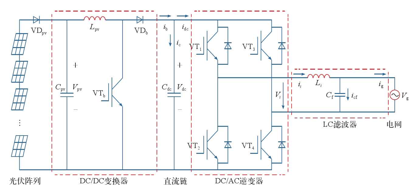
A single-phase two-stage photovoltaic grid connected inverter generally consists of a DC/DC boost circuit and a DC/AC inverter circuit. Compared with single-stage control, although it has a complex structure, its front and rear stages can be controlled separately and are easy to implement; In addition, the front-end DC/DC converter can choose different topology structures according to the input voltage of different solar panels, which is relatively flexible in application compared to single-stage. However, in order to achieve power decoupling between the front and rear stages of a two-stage solar photovoltaic grid connected inverter, a stable DC bus voltage is required.
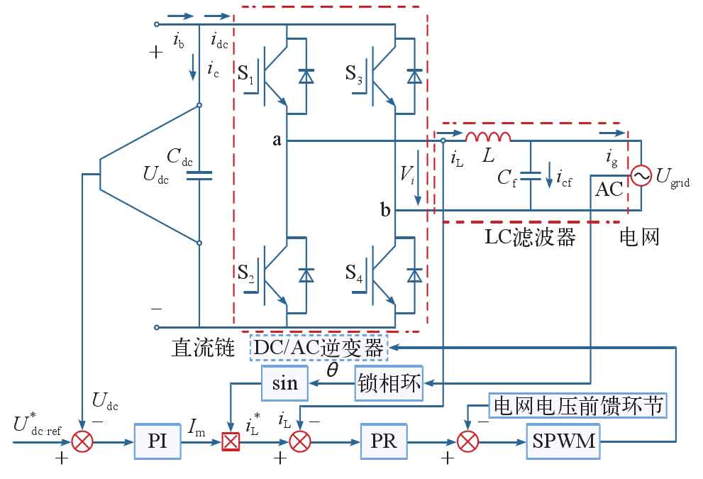
The single-phase two-stage photovoltaic grid connected system diagram is shown in Figure 1. The front stage completes Maximum Power Point Tracking (MPPT), while the rear stage DC/AC needs to take on the task of stabilizing the DC bus voltage and output grid connection.
Due to the fact that the expression of solar panels is a nonlinear time-varying function, and the output of the Boost circuit is obtained through backstage control, there is little literature on front-end modeling, and simulation research based on the Saber platform is scarce. This article takes this as a starting point for step-by-step research and simulation.
1. Establishment of DC/DC level model
Before establishing the front-end model, it is necessary to determine the parameters of the solar panel. Based on the proposed model building method, this paper first builds the output characteristic equation of the photovoltaic panel in Matlab and conducts simulation.
Set the parameters of a single solar panel to Voc=29.2 V. Isc=8.09 V, Vm=23.6 V, Im=7 4 2 A. Among them, Voc is the open circuit voltage of the solar panel; Isc is the short-circuit current of the solar panel; Vm is the voltage at the maximum power point of the solar panel; Im is the current at the maximum power point of the solar panel. Select 10 solar panels as a series, and then connect the three groups in parallel to form a photovoltaic array. The simulation of the P-V characteristic curve of the photovoltaic array is shown in Figure 2.
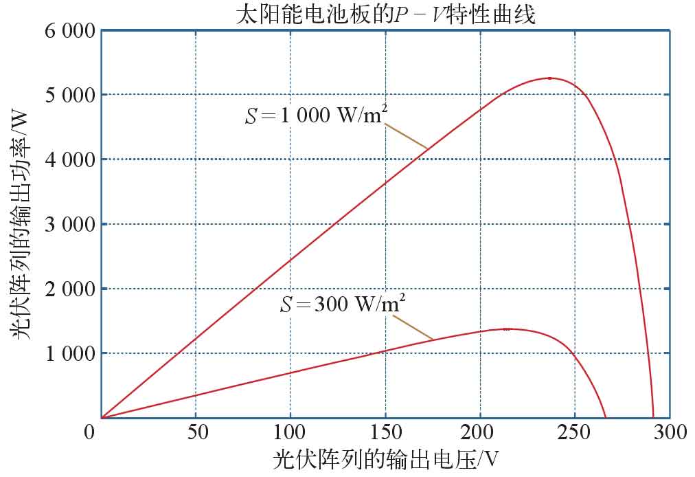
From Figure 2, it can be seen that as the light intensity increases, both the maximum power output and open circuit voltage increase. The output power of the photovoltaic array is approximately 1400 W at a light intensity of 300 W/m2, and approximately 5300 W at 1000 W/m2.
1.1 Establishment of Saber simulation model
The DC/DC converter uses a Boost circuit to achieve MPPT. Since the front-end converter only achieves maximum power output, from another perspective, maximum power point tracking can be achieved by knowing the parameters and configuration of the solar panel in advance, and stabilizing the output voltage of the photovoltaic array at the corresponding value at the maximum power point through loop control. The loop control block diagram is shown in Figure 3.
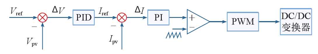
Compare the voltage value Vref corresponding to the maximum power point of the given solar panel with the measured output voltage Vpv of the solar panel. The error is adjusted by PID to obtain the reference value Iref of the solar panel’s output current. Then, compare it with the actual output current, adjust the error by PI, and compare it with the triangular carrier wave to obtain the PWM wave driving the Boost circuit switching transistor. Due to the fact that the bus voltage of the DC/DC converter is regulated by the later stage, a DC source was used in the simulation to represent it.
1.2 Circuit simulation results based on Saber platform
The parameter design of the solar panel is based on the above introduction, and the voltage setting of the solar panel in the simulation is set at 236 V. From Figure 2, it can be seen that there is a slight change in Vm before and after the change in lighting. Ignoring this change, it is set as a constant value. At the beginning, the light intensity was set to 300 W/m ^ 2. After running for 0.5 seconds, it suddenly changed to 1000 W/m ^ 2. The output voltage, current, and power curves of the solar panel are shown in Figure 4.
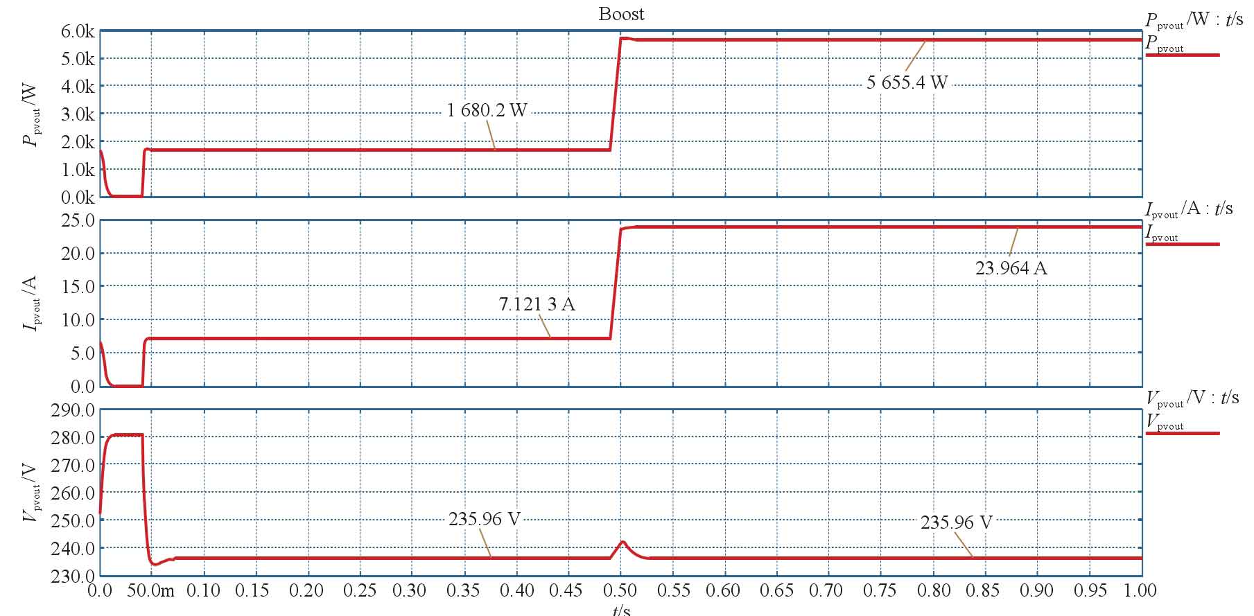
From Figure 4, it can be seen that the output voltage of the solar panel is basically stable at 235.96 V before the change in lighting. After the change in lighting, its output voltage is also stable at 235.96 V. Before the change in lighting, the maximum power tracked by the solar photovoltaic array was measured to be 1688.4 W by loading a horizontal line. After the change in lighting, the stable output power tracked was 5655.4 W, which is slightly larger than the simulation results built in Matlab in Figure 2 by 200 W. The reason is that the engineering model built in Matlab ignored the internal resistance of the photovoltaic panel, and coupled with formula simplification, there will be some error compared to the more accurate model in Saber when the output voltage level is high. But the feasibility and accuracy of this control method can be verified from the results.
2. Control strategy for inverter grid connection
The DC-AC part of the later stage uses a single-phase full bridge circuit to transmit power from the solar photovoltaic inverter to the grid. According to the requirements of grid connection for the output of solar photovoltaic inverters, this article adopts a dual closed-loop control method. Although traditional dual loop control based on PI and PR regulation is simple, PI control is difficult to achieve control effect on sinusoidal reference current. When the capacitance of the output filter is large, the system may experience oscillation. Therefore, to overcome its shortcomings, a loop control structure based on proportional resonance (PR) regulation is adopted.
2.1 Control methods for inverter circuits
The outer loop of the double closed loop is controlled by DC voltage, and the balance of input and output energy of the solar photovoltaic inverter is achieved by adjusting the stable DC side voltage through PI; The current amplitude reference value Im * of the inner current loop is given by the output of the DC voltage outer loop regulator, and the phase angle of the grid voltage is obtained through detection θ, And by sin θ、 The product of Im * obtains the reference signal IL * for the instantaneous output current. In order to suppress the disturbance of the grid voltage, grid voltage feedforward control is adopted. After the output of the current loop is superimposed with the feedforward signal of the grid voltage, the driving signal is modulated by SPWM to control the switch of the inverter bridge, in order to achieve grid connection control of the single-phase solar photovoltaic inverter. The system control block diagram is shown in Figure 5.
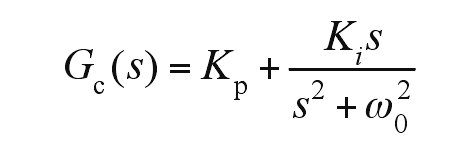
The transfer function of the PR regulator is:
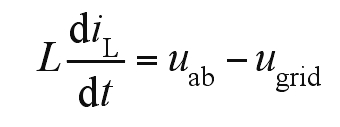
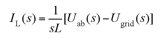
Ignoring the internal resistance and switching losses of the circuit, iL is taken as the state variable from Figure 5, and there is a basic relationship formula, which is:
According to the modulation principle, it can be concluded that:
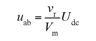
In the formula, vr is the sine wave modulation wave of the solar photovoltaic inverter; Vm is the amplitude of the high-frequency triangular carrier wave.
Performing Laplace transformation on the formula yields:
Construct a closed-loop transfer function for the system, as shown in Figure 6.
Without considering the influence of grid voltage, set the DC bus voltage to 360 V and the inverter inductance to 1100 μ F. The sampling multiple is 0.05, the amplitude of the triangular carrier is 3, and the PI and PR parameters are adjusted. The transfer function of the current loop is:
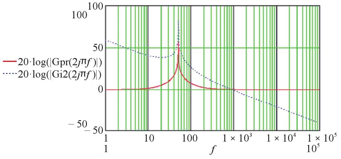
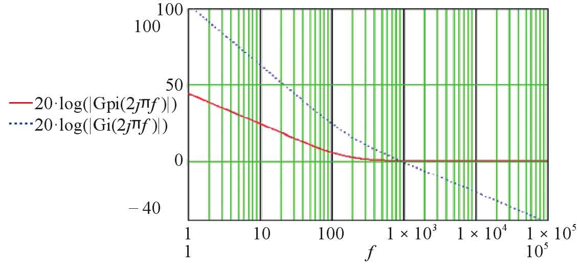
Find its Bode diagram, as shown in Figures 7 and 8.
2.2 System modeling and simulation results
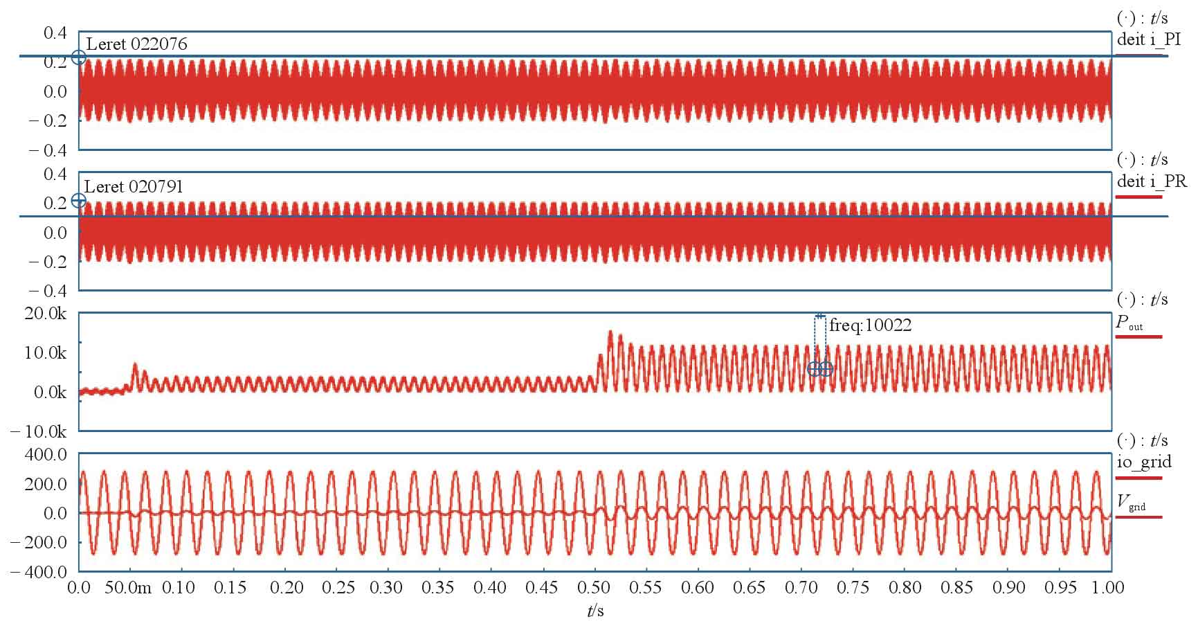
Based on the control method of the previous Boost circuit and the control block diagram shown in Figure 6, a Saber simulation model is constructed for the entire system. The output result after system operation is shown in Figure 9. It can be seen that the controlled inductor current can quickly and stably operate after one cycle of adjustment after the occurrence of light disturbance. The average error between the actual inductor current and the given current is almost zero, while the output of the current loop error based on PI adjustment is a differential envelope cycle function. The new control method has a fast dynamic response, with a stable grid connected current and power.
3. Conclusion
By building and simulating an engineering application model of solar panels in Matlab, the maximum output power under different lighting conditions is obtained. Based on this data background, modeling and simulation of single-phase two-stage solar photovoltaic grid connected inverters were carried out step by step using Saber software. The front-end Boost circuit adopts the voltage at the predetermined optimal point, and obtains the maximum power output through the control mode of voltage outer loop and current inner loop. From the simulation results, it can be seen that this method achieves maximum power tracking of the solar panel; The later stage DC/AC utilizes a full bridge inverter circuit and compares the error between the controlled quantity and the sampling value obtained by traditional PI and PR adjustment methods. It can be concluded that changing to PI and PR adjustment can effectively achieve zero static error control of grid connected current. Finally, this method was adopted to achieve stable tracking of the frequency and phase of the grid voltage for the output of the solar photovoltaic inverter, meeting the requirements of grid connection for the solar photovoltaic inverter. Especially when the lighting changes, it can quickly and accurately adjust the grid connection, thus verifying the feasibility of the control method used in the system.