
I treat the grid-connected solar inverter as the decisive interface between a photovoltaic array and the utility network. In my study, solar inverters must convert DC power into AC power while also shaping the current so that the point of common coupling remains within harmonic limits. Because nonlinear loads and many power electronic devices inject harmonic currents into the distribution network, the power quality problem is not only a converter problem; it is a system problem. I therefore focus on the current control strategy of solar inverters, because the current loop determines harmonic suppression, tracking accuracy, transient speed, and robustness.
I start from the fact that a solar inverter is not an ideal current source. Its switching process creates high-frequency harmonics, its filter creates a resonant peak, and its controller must reject grid-voltage distortion and DC-link variation. In my design, I compare filter topologies, establish a three-phase LCL model, design the filter parameters, and then compare repetitive control, sliding mode control, and a weighted hybrid control strategy. The final objective is a solar inverter current loop that keeps total harmonic distortion low, tracks the fundamental reference with small error, and remains stable when operating conditions change.
I summarize the common harmonic-current limits that guide my design in Table 1. These limits are not the only criterion, but they provide a clear boundary for acceptable grid-connected current quality.
| Harmonic order | Limit as a percentage of fundamental |
|---|---|
| Odd harmonics below 11 | Less than 4% |
| 11 to 16 | Less than 2% |
| 17 to 22 | Less than 1.5% |
| 23 to 34 | Less than 0.6% |
| 35 and above | Less than 0.3% |
| Total harmonic distortion | Less than 5% |
The total harmonic distortion of current is defined as
$$ \mathrm{THD}_I=\frac{I_H}{I_1}\times 100\% $$
where $$ I_H $$ is the root-mean-square value of the harmonic current and $$ I_1 $$ is the root-mean-square value of the fundamental current. The harmonic current content is
$$ I_H=\sqrt{\sum_{n=2}^{\infty} I_n^2} $$
where $$ I_n $$ is the effective value of the nth harmonic current. I use these definitions repeatedly when I judge whether a solar inverter is suitable for grid connection.
I first compare the L filter, the LC filter, and the LCL filter. The L filter is a first-order filter, and its transfer function from inverter voltage to grid current is
$$ G_L(s)=\frac{i_2(s)}{u_{inv}(s)}=\frac{1}{Ls} $$
The L filter attenuates high-frequency components at 20 dB per decade, which is often insufficient for modern solar inverters with high switching frequency and strict harmonic limits. The LC filter can attenuate switching harmonics, but its capacitor branch can resonate with the grid impedance, so I do not prefer it for a grid-connected solar inverter. The LCL filter provides third-order attenuation and can reduce switching harmonics more effectively with smaller total inductance. Its ideal transfer function is
$$ G_{LCL}(s)=\frac{i_2(s)}{u_{inv}(s)}=\frac{1}{L_1L_2Cs^3+(L_1+L_2)s} $$
The LCL filter has a resonant peak. If I do not damp this peak, the solar inverter current loop can become unstable or oscillatory. I therefore compare passive damping positions and select a practical damping method. In Table 2, I summarize the qualitative comparison of the three filter types.
| Filter type | Order | High-frequency attenuation | Main advantage | Main drawback |
|---|---|---|---|---|
| L | First order | 20 dB per decade | Simple and robust | Large inductance and weak harmonic attenuation |
| LC | Second order | 40 dB per decade | Good attenuation | Resonance with grid impedance |
| LCL | Third order | 60 dB per decade | Smaller total inductance and strong harmonic suppression | Resonant peak and more complex control |
I examine six passive damping positions: series and parallel resistance on the inverter-side inductor, series and parallel resistance on the grid-side inductor, and series and parallel resistance on the filter capacitor. I summarize the behavior in Table 3.
| Damping position | Effect on resonant peak | Effect on low-frequency gain | Loss consideration |
|---|---|---|---|
| Series resistance with $$ L_1 $$ | Reduces peak | Reduces low-frequency gain | Higher current loss |
| Parallel resistance with $$ L_1 $$ | Reduces peak | Weakens low-frequency behavior | Poor high-frequency attenuation |
| Series resistance with $$ L_2 $$ | Reduces peak | Affects high-frequency attenuation | Higher harmonic loss |
| Parallel resistance with $$ L_2 $$ | Reduces peak | Weakens high-frequency attenuation | Loss depends on grid-side current |
| Series resistance with $$ C $$ | Strong peak reduction | Almost unchanged low-frequency gain | Low loss because capacitor current is mostly high frequency |
| Parallel resistance with $$ C $$ | Reduces peak | Low-frequency gain unchanged | High loss because capacitor voltage is large |
From my comparison, I select a series resistor in the capacitor branch. This damping method suppresses the LCL resonant peak while preserving the low-frequency gain. The capacitor branch carries mainly high-frequency current, so the resistor loss is lower than in the parallel-capacitor case. The transfer function of the damped LCL filter becomes
$$ G_{LCL,RC}(s)=\frac{sCR_C+1}{L_1L_2Cs^3+(L_1+L_2)CR_Cs^2+(L_1+L_2)s} $$
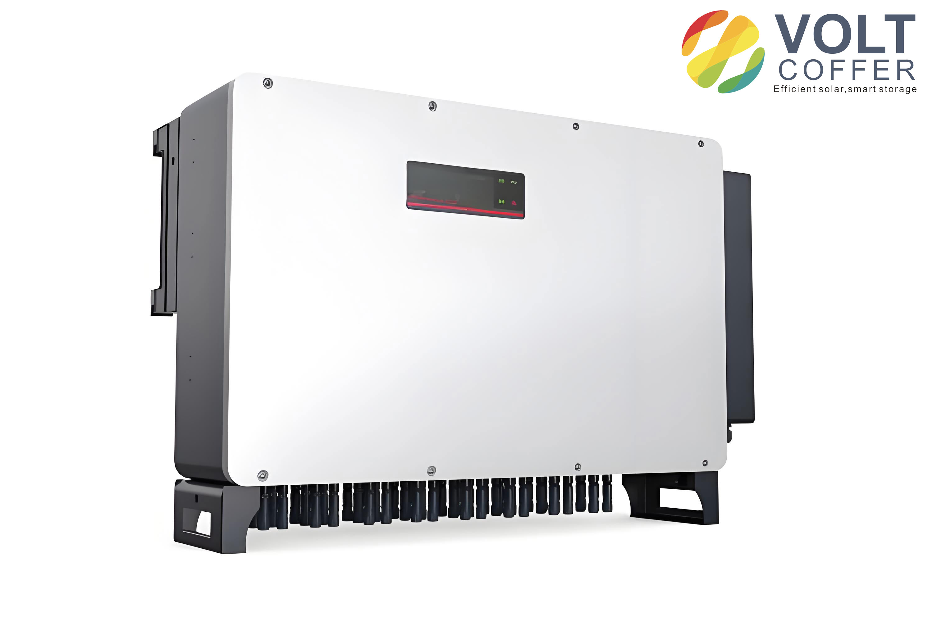
I use this damped LCL network as the plant for my solar inverter current controller. The hardware arrangement also reflects the practical structure of a three-phase solar inverter, as shown in the inserted image.
After selecting the LCL filter, I build the three-phase mathematical model. The inverter-side current is $$ i_a,i_b,i_c $$, the capacitor voltage is $$ u_{ca},u_{cb},u_{cc} $$, the grid-side current is $$ i_{ga},i_{gb},i_{gc} $$, and the grid voltage is $$ u_{ga},u_{gb},u_{gc} $$. The state equations in the stationary abc frame are
$$ L_1\frac{di_a}{dt}=u_{dc}-u_{ca} $$
$$ L_1\frac{di_b}{dt}=u_{dc}-u_{cb} $$
$$ L_1\frac{di_c}{dt}=u_{dc}-u_{cc} $$
$$ C\frac{du_{ca}}{dt}=i_a-i_{ga} $$
$$ C\frac{du_{cb}}{dt}=i_b-i_{gb} $$
$$ C\frac{du_{cc}}{dt}=i_c-i_{gc} $$
$$ L_2\frac{di_{ga}}{dt}=u_{ca}-u_{ga} $$
$$ L_2\frac{di_{gb}}{dt}=u_{cb}-u_{gb} $$
$$ L_2\frac{di_{gc}}{dt}=u_{cc}-u_{gc} $$
Because the currents and voltages are AC quantities in the stationary frame, I apply the Park transformation to obtain DC quantities in the synchronous rotating dq frame. The transformation matrix is
$$ T_{3s/2r}=\frac{2}{3}\begin{bmatrix} \cos\theta & \cos(\theta-\frac{2\pi}{3}) & \cos(\theta+\frac{2\pi}{3}) \\ -\sin\theta & -\sin(\theta-\frac{2\pi}{3}) & -\sin(\theta+\frac{2\pi}{3}) \end{bmatrix} $$
With $$ \theta=\omega t $$ and $$ \omega=2\pi f_0 $$, the LCL solar inverter model in the dq frame becomes
$$ L_1\frac{di_d}{dt}=u_d-u_{cd}+\omega L_1i_q $$
$$ L_1\frac{di_q}{dt}=u_q-u_{cq}-\omega L_1i_d $$
$$ C\frac{du_{cd}}{dt}=i_d-i_{gd}+\omega Cu_{cq} $$
$$ C\frac{du_{cq}}{dt}=i_q-i_{gq}-\omega Cu_{cd} $$
$$ L_2\frac{di_{gd}}{dt}=u_{cd}-u_{gd}+\omega L_2i_{gq} $$
$$ L_2\frac{di_{gq}}{dt}=u_{cq}-u_{gq}-\omega L_2i_{gd} $$
These equations show cross-coupling between the d and q axes. I must decouple these terms in the current controller. I also use the active and reactive power relations. If the grid voltage is aligned with the d axis, then $$ u_{gq}=0 $$, and the powers are
$$ P=\frac{3}{2}u_{gd}i_d $$
$$ Q=\frac{3}{2}u_{gd}i_q $$
Thus, I can control active power by controlling $$ i_d $$ and reactive power by controlling $$ i_q $$. This is why the current control loop of a solar inverter is usually designed in the dq frame.
I next design the LCL parameters. The inverter-side inductance must limit the switching ripple. If the maximum ripple is required to stay below 15% of the rated current peak, then the lower bound is
$$ L_{1,\min}=\frac{U_{dc}}{4\times 15\%\times I_n f_{kg}} $$
where $$ U_{dc} $$ is the DC-link voltage, $$ I_n $$ is the rated current peak, and $$ f_{kg} $$ is the switching frequency. The total inductance must not create excessive voltage drop. I choose the upper bound as
$$ L_{T,\max}=\frac{10\%U_g}{2\pi f_0 I_g} $$
Then the inverter-side inductance must satisfy
$$ L_{1,\min}\le L_1\le L_{T,\max} $$
The grid-side inductance is usually chosen with a ratio between the inverter-side and grid-side inductances:
$$ L_1=\nu L_2,\quad 3<\nu<7 $$
Therefore,
$$ L_2=\frac{L_1}{\nu} $$
The filter capacitor must not consume too much reactive power. I require the capacitor reactive power to remain below 5% of the rated active power:
$$ \omega_0 C U_C^2\le 5\%P_N $$
Because the grid-side inductance is small, I approximate the capacitor voltage by the grid voltage. The maximum capacitance is
$$ C_{\max}=\frac{5\%P_N}{\omega_0 U_g^2} $$
The resonance frequency must be placed between the fundamental frequency and the switching frequency. I use the constraint
$$ 10f_0<f_x<0.5f_{kg} $$
where
$$ f_x=\frac{1}{2\pi}\sqrt{\frac{L_1+L_2}{L_1L_2C}} $$
I summarize my chosen parameters in Table 4.
| Parameter | Symbol | Value |
|---|---|---|
| DC-link voltage | $$ U_{dc} $$ | 600 V |
| Grid voltage | $$ U_g $$ | 220 V |
| Fundamental frequency | $$ f_0 $$ | 50 Hz |
| Switching frequency | $$ f_{kg} $$ | 10 kHz |
| Inverter-side inductance | $$ L_1 $$ | 2 mH |
| Grid-side inductance | $$ L_2 $$ | 0.4 mH |
| Filter capacitance | $$ C $$ | 11 microfarad |
| Resonance frequency | $$ f_x $$ | About 2.63 kHz |
I check the resonance constraint. With my parameters, the resonance frequency is about 2.63 kHz, which is greater than 500 Hz and less than 5 kHz, so the design satisfies the constraint. This parameter set forms the basis of my solar inverter simulations.
I then design the repetitive controller. Repetitive control is based on the internal model principle. If a signal repeats every period, the controller can place a model of that periodic signal inside the closed loop. The continuous internal model is
$$ G_{rc}(s)=\frac{e^{-sT}}{1-e^{-sT}} $$
In discrete time, I use
$$ G_{rc}(z)=\frac{z^{-N}}{1-Q(z)z^{-N}} $$
where $$ N $$ is the number of samples in one fundamental period and $$ Q(z) $$ is a filter or a constant slightly less than one. I set $$ Q(z)=0.95 $$ to improve stability. The term $$ z^{-N} $$ introduces a delay of one fundamental period. This delay is the main reason why a pure repetitive controller has slow transient response. The controller cannot correct an error in the present period until the next period.
To improve the dynamic response, I combine repetitive control with proportional-integral control. The proportional-integral part acts quickly when the error first appears, while the repetitive part eliminates periodic error over successive cycles. The compensation block is
$$ C(z)=K_rz^kS(z) $$
where $$ K_r $$ is the repetitive gain, $$ z^k $$ is a phase-lead term, and $$ S(z) $$ is a low-pass filter. I choose $$ K_r=1 $$, $$ k=4 $$, and a second-order low-pass filter:
$$ S(s)=\frac{\omega_n^2}{s^2+2\xi\omega_ns+\omega_n^2} $$
I set the cutoff frequency to 650 Hz, so $$ \omega_n=4084 $$ rad/s. I choose $$ \xi=0.8 $$ to reduce overshoot while keeping a fast response. The discrete form is
$$ S(z)=\frac{0.067z-0.0538}{z^2-1.3995z+0.5203} $$
The stability condition for the repetitive controller can be written as
$$ |Q(e^{j\omega T})-K_re^{jk\omega T}S(e^{j\omega T})P(e^{j\omega T})|<1 $$
for all frequencies. This condition means that the vector representing the compensated plant must remain inside a unit circle centered at $$ Q(e^{j\omega T}) $$. When $$ Q $$ is slightly less than one, the circle shifts to the left, which improves robustness in the middle- and high-frequency ranges.
I design the proportional-integral part with $$ K_p=10 $$ and $$ K_i=100 $$. The composite controller in the dq frame decouples the axes using
$$ u_d=K_p(i_d^*-i_d)+\frac{K_i}{s}(i_d^*-i_d)+u_{gd}-\omega Li_q $$
$$ u_q=K_p(i_q^*-i_q)+\frac{K_i}{s}(i_q^*-i_q)+u_{gq}+\omega Li_d $$
where $$ L=L_1+L_2 $$. The repetitive block is added in parallel with this proportional-integral structure. I summarize the controller parameters in Table 5.
| Controller parameter | Value |
|---|---|
| Proportional gain $$ K_p $$ | 10 |
| Integral gain $$ K_i $$ | 100 |
| Repetitive gain $$ K_r $$ | 1 |
| Internal model filter $$ Q $$ | 0.95 |
| Samples per period $$ N $$ | 200 |
| Phase lead $$ k $$ | 4 |
| Low-pass filter cutoff | 650 Hz |
| Damping ratio $$ \xi $$ | 0.8 |
I simulate the proportional-integral controller and the repetitive proportional controller. Under proportional-integral control alone, the solar inverter current settles slowly and the error remains noticeable for a long time. Under the repetitive proportional controller, the current error converges much faster and the steady-state error becomes very small. I compare the two cases in Table 6.
| Control method | Tracking speed | Steady-state error | Periodic disturbance rejection | Transient behavior |
|---|---|---|---|---|
| Proportional-integral | Moderate | Small but not zero for AC reference | Limited | Fast initial action but no periodic learning |
| Repetitive proportional | Slower first cycle due to delay | Very small after several cycles | Strong | One-period delay in learning |
Although the repetitive proportional controller performs well in steady state, its delay causes a slow first-cycle response. I therefore study sliding mode control as a second candidate. Sliding mode control is a nonlinear control method that changes the structure of the controller according to the system state. Its main advantage is robustness to parameter variation and external disturbance. I consider a system
$$ \dot{x}=Ax+Bu $$
and define a sliding surface
$$ s(x)=C^Tx=c_1x_1+c_2x_2+\cdots+x_n $$
where the coefficients are chosen so that the sliding polynomial is Hurwitz. The control law drives the state to the sliding surface and then keeps it on that surface. I analyze three common reaching laws in Table 7.
| Reaching law | Expression | Property |
|---|---|---|
| Constant reaching law | $$ \dot{s}=-\epsilon\mathrm{sgn}(s),\epsilon>0 $$ | Simple; larger $$ \epsilon $$ gives faster reaching but more chattering |
| Exponential reaching law | $$ \dot{s}=-ks-\epsilon\mathrm{sgn}(s),k>0,\epsilon>0 $$ | Fast reaching and reduced reaching time |
| Power reaching law | $$ \dot{s}=-k|s|^\alpha\mathrm{sgn}(s),k>0,0<\alpha<1 $$ | Large reaching speed far from the surface and smaller gain near the surface |
Sliding mode control has three important properties: reachability, stability, and invariance. Reachability means that the state can reach the sliding surface in finite time. Stability means that the sliding motion is stable after the state reaches the surface. Invariance means that the sliding mode is insensitive to matched parameter variations and disturbances. However, sliding mode control has an inherent chattering problem. The switching function is discontinuous, and in a real digital implementation the state cannot switch infinitely fast. The result is a high-frequency oscillation around the sliding surface. Causes of chattering include switching delay, spatial hysteresis, system inertia, and discrete sampling. I summarize these causes in Table 8.
| Cause of chattering | Explanation | Effect on a solar inverter |
|---|---|---|
| Switching delay | Control action is not applied at the exact crossing instant | High-frequency current ripple |
| Spatial hysteresis | A dead zone exists near the switching surface | Oscillation of the current error |
| System inertia | The plant cannot change its state instantly | Overshoot and residual oscillation |
| Discrete sampling | The controller updates only at sampling instants | Quasi-sliding motion and bounded chattering |
To reduce chattering, I replace the sign function with a high-frequency smoothing function. The conventional switching term is
$$ u_{SM}(s)=\rho\frac{s}{|s|} $$
I use instead
$$ u_{HF}(s)=\rho\frac{s}{|s|+\epsilon} $$
This function is continuous and reduces the abrupt switching action. When $$ \epsilon=0 $$, it becomes the sign function. When $$ \epsilon>0 $$, the magnitude of the control near the sliding surface is reduced. I apply this improved reaching law to the d and q axes. I define the tracking errors as
$$ e_d=i_d^*-i_d $$
$$ e_q=i_q^*-i_q $$
I define the sliding surfaces as
$$ s_d=ce_d+\int_0^t e_d\,dt $$
$$ s_q=ce_q+\int_0^t e_q\,dt $$
with $$ c>0 $$. Then
$$ \dot{s}_d=c\dot{e}_d+e_d $$
$$ \dot{s}_q=c\dot{e}_q+e_q $$
I choose the reaching laws
$$ \dot{s}_d=-u_{HF}(s_d)-e_d $$
$$ \dot{s}_q=-u_{HF}(s_q)-e_q $$
I define a Lyapunov function
$$ V=\frac{1}{2}s_d^2+\frac{1}{2}s_q^2 $$
Its derivative is
$$ \dot{V}=s_d\dot{s}_d+s_q\dot{s}_q=-s_d u_{HF}(s_d)-s_q u_{HF}(s_q)\le 0 $$
Thus, the sliding-mode current loop is stable in the Lyapunov sense. The d-axis current tracking under sliding mode control converges quickly, but the error still shows chattering because the switching term cannot be perfectly smooth. I summarize the sliding mode controller parameters in Table 9.
| Sliding mode parameter | Value or condition |
|---|---|
| Sliding surface coefficient $$ c $$ | Positive constant |
| Reaching gain $$ \rho $$ | Positive constant |
| Smoothing factor $$ \epsilon $$ | Small positive constant |
| Lyapunov function | $$ V=\frac{1}{2}s_d^2+\frac{1}{2}s_q^2 $$ |
| Stability condition | $$ \dot{V}\le 0 $$ |
My simulations show that sliding mode control gives a faster initial tracking response than the repetitive proportional controller, but the steady-state current error oscillates more. The repetitive proportional controller gives a smoother steady-state current, but its first-cycle response is slower. This trade-off leads me to a weighted hybrid control strategy. I combine the repetitive proportional controller and the sliding mode controller by a time-varying weight. The weighted control law is
$$ u_d=aG(s)e_d+(1-a)u_{HF}(s_d)-Ri_d+u_{gd}-\omega Li_q $$
$$ u_q=aG(s)e_q+(1-a)u_{HF}(s_q)-Ri_q+u_{gq}+\omega Li_d $$
where $$ G(s) $$ is the repetitive proportional controller, $$ a $$ is the weight, and $$ 0\le a\le 1 $$. When the current error is large, I set $$ a=0 $$ so that the sliding mode controller dominates and drives the error down quickly. When the current error becomes small, I increase $$ a $$ so that the repetitive proportional controller dominates and provides a smooth steady state. I design the weight as
$$ a=0\quad\mathrm{when}\ |e|>\eta_2 $$
$$ a=\mathrm{roundn}(|e|,2)\frac{\mu(\eta_2-|e|)}{2(\eta_2-\eta_1)}\quad\mathrm{when}\ \eta_1<|e|\le\eta_2 $$
$$ a=\mu\quad\mathrm{when}\ |e|\le\eta_1 $$
where $$ \eta_1 $$ and $$ \eta_2 $$ are the lower and upper error thresholds, $$ \mu $$ is the maximum weight, and $$ \mathrm{roundn}(|e|,2) $$ rounds the error to two decimal places. I summarize the weight logic in Table 10.
| Error condition | Weight $$ a $$ | Dominant controller | Purpose |
|---|---|---|---|
| $$ |e|>\eta_2 $$ | 0 | Sliding mode | Fast error reduction |
| $$ \eta_1<|e|\le\eta_2 $$ | Gradually increasing | Mixed | Smooth transition |
| $$ |e|\le\eta_1 $$ | $$ \mu $$ | Repetitive proportional | Low steady-state error and low chattering |
I test the weighted hybrid control in the same solar inverter simulation model. I use a fixed-step solver, a simulation time of 0.25 s, and a step size of $$ 1\times10^{-6} $$ s. The DC-link voltage is 600 V, the AC grid voltage is 380 V, the switching frequency is 10 kHz, the inverter-side inductance is 2 mH, the grid-side inductance is 0.4 mH, and the filter capacitance is 11 microfarad. I compare three cases: repetitive proportional control, sliding mode control, and weighted hybrid control. The comparison is summarized in Table 11.
| Control method | Approximate settling time | Current error range | Waveform smoothness | Robustness |
|---|---|---|---|---|
| Repetitive proportional | About 0.18 s | About 0 to 2 A after settling | Very smooth | Good for periodic disturbance |
| Sliding mode | About 0.003 s | About 0 to 2.3 A with chattering | Visible chattering and spikes | Strong against parameter variation |
| Weighted hybrid | About 0.003 s | About 0 to 2 A | Smooth after transition | Strong and smooth |
The weighted hybrid controller reaches the steady state almost as fast as the sliding mode controller and keeps the steady-state error as small as the repetitive proportional controller. The grid current remains sinusoidal, and the voltage and current are in phase. I also perform a fast Fourier transform analysis. The results are shown in Table 12.
| Control method | Fundamental amplitude | Total harmonic distortion |
|---|---|---|
| Repetitive proportional | 23.29 | 4.02% |
| Sliding mode | 21.05 | 2.60% |
| Weighted hybrid | 21.10 | 2.51% |
The weighted hybrid control gives the lowest total harmonic distortion among the three cases. I also test the robustness of the weighted hybrid control by changing the DC-link voltage from 600 V to 700 V at 0.1 s. The current error recovers quickly, and the grid current remains smooth. This shows that the weighted hybrid control preserves the fast response of sliding mode control and the steady-state quality of repetitive proportional control. I summarize the robustness test in Table 13.
| Disturbance | Time of change | Recovery behavior | Current waveform |
|---|---|---|---|
| DC-link voltage step 600 V to 700 V | 0.1 s | Error returns to a small band quickly | Remains smooth and in phase with voltage |
From my point of view, the main contribution of this work is the combination of a repetitive proportional controller and a sliding mode controller through a real-time weight. The weighted controller allows solar inverters to use sliding mode control during large transients and repetitive proportional control during steady-state operation. This avoids the slow first-cycle response of pure repetitive control and the high chattering of pure sliding mode control. The resulting solar inverter current loop has low harmonic distortion, fast dynamic response, and good robustness.
I also note several limitations that I would investigate further. First, I have considered a three-phase balanced system. The behavior of solar inverters under unbalanced or distorted grid conditions requires additional study. Second, I have treated the DC side as a stiff voltage source. In a real solar inverter, the front-end DC-DC converter and the maximum power point tracking loop interact with the inverter current loop. Third, I have not included local nonlinear loads in the simulation. If nonlinear loads are connected near the solar inverter, the harmonic current compensation problem becomes more complex. These issues are important for future work because solar inverters are increasingly expected to support power quality, not merely inject active power.
In my final assessment, the LCL filter with capacitor-series passive damping provides a suitable plant for a grid-connected solar inverter. The repetitive proportional controller provides strong periodic error suppression. The sliding mode controller provides fast transient response and robustness. The weighted hybrid controller combines both advantages. The simulation results show that the weighted hybrid control keeps the current error small, reduces total harmonic distortion to about 2.51%, and recovers quickly after a DC-link voltage step. I therefore conclude that the weighted hybrid control strategy is a practical and effective method for improving the current quality and dynamic performance of solar inverters connected to the grid.