
Battery energy storage systems will not be infinitely configured in practical applications, and its capacity configuration is closely related to the economy of microgrids. The economy of microgrids belongs to nonlinear problems; It is best to use intelligent algorithms to quickly and accurately solve this problem in order to quickly find the optimal solution. At present, traditional intelligent algorithms have a relatively large capacity when solving the capacity allocation of battery energy storage systems. Therefore, it is necessary to solve nonlinear problems with two or more intelligent algorithms to improve the algorithm’s optimization ability in order to find the optimal solution for capacity allocation. This chapter establishes an economic model for the battery energy storage systems peak shaving and valley filling DC microgrid based on the constraints of battery energy storage systems charging and discharging limits, load shortage rate, and battery energy storage system overcharging and discharging. In response to the problem of poor convergence and low solving accuracy of the Artificial Bee Colony Algorithm (ABC), multiple search strategies have been integrated into the ABC algorithm, which improve the problem of poor convergence and low solving accuracy of the ABC algorithm. The improved ABC algorithm was tested through testing functions, and the optimal configuration of battery energy storage systems capacity was obtained through non-linear optimization of capacity optimization configuration in battery energy storage systems microgrids.
1. Random production simulation method
The traditional battery energy storage systems capacity configuration method is the random simulation production method. The random simulation production method [50-51] is based on the power load prediction curve, the start/stop of generator units, and the fluctuation of new energy generation, which are equivalent to the continuous load curve. Based on the two indicators of Loss of Load Probability (LOLP) and Expected Energy not Served (EENS), the required capacity and power for the microgrid battery energy storage systems are obtained, N is the number of units.
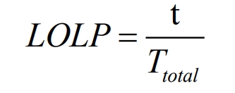
In the formula: 𝑡 is the time when the load power exceeds the maximum total power generated by the microgrid system; 𝑇𝑡𝑜𝑡𝑎𝑙 is the time (𝑇) for randomly simulating production.
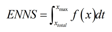
In the formula: 𝑥𝑚𝑎𝑥 is the equivalent maximum power of the load; 𝑥𝑡𝑜𝑡𝑎𝑙 is the maximum total power generated by the system; 𝑓 (𝑥) is the relationship between the load curve and time.
Due to the capacity configuration of LOLP and ENNS, the battery energy storage systems charging and discharging power and capacity were solved, resulting in two different sets of solutions. Not only does it require comparing the two sets of different charging and discharging power and capacity, but the capacity configuration under this method particularly depends on the accuracy of the power load curve. So this article uses intelligent algorithms to solve the objective function for capacity allocation of battery energy storage systems.
2. Battery energy storage system capacity configuration model
2.1 Objective function
The economic model of battery energy storage systems mainly consists of the following four parts: equipment investment cost, daily maintenance cost, low storage and high yield, and government subsidies.
(1) Equipment investment cost
It can be seen that battery energy storage systems is mainly composed of energy storage batteries, inverters, transformers, control units, and BMS, and the investment cost of these equipment constitutes the equipment investment cost of battery energy storage systems. The cost of control units is related to the size of power, which is called power investment cost; The cost of energy storage batteries is related to the size of their capacity, known as energy investment cost. Therefore, the power investment cost and energy investment cost of battery energy storage systems constitute the equipment investment cost of battery energy storage systems. The investment cost is shown in the formula.
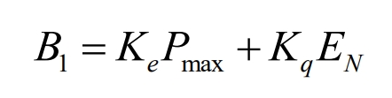
In the formula, 𝐵 1 is the equipment investment cost of battery energy storage systems; 𝐾𝑒 Cost coefficient of power components per unit power (kW/yuan); 𝑃𝑚𝑎𝑥 is the maximum power value of the power element (control unit); 𝐾𝑞 is the battery energy storage systems capacity cost coefficient (kWh/yuan); 𝐸𝑁 is the rated power of the energy element (energy storage battery).
(2) Daily operation and maintenance costs
In the practical application of battery energy storage systems in microgrids, daily maintenance and service life reduction are required; The maintenance of equipment in battery energy storage systems is called the maintenance cost of battery energy storage systems, and the service life depreciation cost of equipment in battery energy storage systems is called the operating cost of battery energy storage systems. The daily operation and maintenance cost of battery energy storage systems is composed of maintenance cost and service life depreciation cost, as shown in the formula.
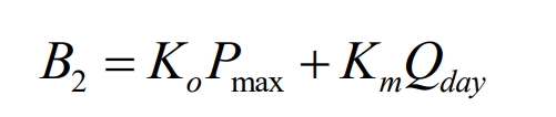
In the formula, 𝐵 2 is the daily operation and maintenance cost of battery energy storage systems; 𝐾𝑜 is the daily operating cost coefficient of power components within a unit power (kW/yuan); 𝐾𝑚 is the maintenance cost coefficient of capacity components per unit capacity (kWh/yuan); 𝑄𝑑𝑎𝑦 is the daily discharge capacity (kWh) of battery energy storage systems.
(3) Low storage and high yield
When the power load is at its peak, it is necessary to increase the installed capacity of the generator set, resulting in an increase in power generation cost per unit time, which is uneconomical. However, during the low peak of the power load, a large number of units will start and stop, reducing the power generation capacity of the generator set. The energy consumption increases in increments, resulting in a waste of manpower and material resources, which is neither economic nor environmentally friendly. Using battery energy storage systems to discharge during peak power loads, achieving the goal of peak power load reduction; Charging during low power load periods achieves the goal of peak load filling, thereby achieving peak load shaving and valley filling. Therefore, it brings low storage and high generation benefits to the microgrid; During peak power load, battery energy storage systems sells electricity to the microgrid at a higher price; When the power load is low, battery energy storage systems charges at a lower electricity price, utilizing the differences in electricity prices at different time periods to achieve the benefits of low storage and high generation in the microgrid, as shown in the formula.
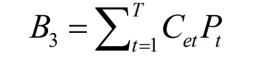
In the formula, 𝐵 3 represents the return on low storage and high issuance of battery energy storage systems; 𝐶𝑒𝑡 is the electricity price at the specified time; 𝑃𝑐𝑡 is the charging and discharging power of the battery energy storage systems at a certain time, with 𝑃𝑡>0 during battery energy storage systems discharge and 𝑃𝑡<0 during battery energy storage systems charging.
(4) Government subsidies
In order to support the widespread use of battery energy storage systems, the government has introduced an economic subsidy policy for battery energy storage systems installed capacity, as shown in the formula.
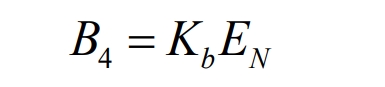
In the formula, 𝐵 4 represents government subsidies; 𝐾𝑏 is the subsidy coefficient of capacity components per unit capacity (kWh/yuan);
𝐸𝑁 is the rated capacity of battery energy storage systems.
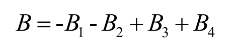
In summary, the economic benefits brought by battery energy storage systems to the power grid are composed of two parts: B3 and B4, while the economic benefits of the power grid are composed of four parts: 𝐵 1, 𝐵 2, 𝐵 3, and 𝐵 4. Therefore, the economic expression of the power grid is shown in the formula.
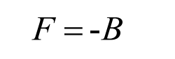
In order to facilitate the improvement of particle swarm optimization algorithm, the objective function 𝐹 1 is shown in the formula.
2.2 Constraints
In the process of battery energy storage systems configuration, it is necessary to consider the influence of its performance constraints, charging and discharging power constraints, and the battery energy storage systems life model.
(1) SOC constraints
During the charging and discharging process of battery energy storage systems, it is necessary to consider the impact of overcharging and discharging on the lifespan of battery energy storage systems. Usually, a range needs to be set for 𝑆𝑂𝐶, as shown in the formula.
(2) The charging and discharging constraints of BESS are shown in the formula.
In the formula, 𝑃𝑐 is the charging power of battery energy storage systems, 𝑃𝑑 is the discharge power of battery energy storage systems, and 𝑃𝑒 is the rated power of battery energy storage systems.
(3) Load shortage rate 𝑓
The load shortage rate 𝑓 is the ratio of insufficient power supply to the total electricity required by the power load, as shown in the formula. 𝑓 to a certain extent, it reflects the reliability of microgrid power supply. A larger 𝑓 indicates a poorer power supply reliability, while a smaller 𝑓 value indicates a higher power supply reliability. Therefore, it is necessary to set an upper limit for the load to ensure that the load fluctuates within a certain range.
In the formula, 𝐸𝑙𝑎𝑐𝑘 represents insufficient power supply; 𝐸𝑜𝑣𝑒𝑟𝑎𝑙𝑙 is the total amount required for power load; 𝑓𝑚𝑎𝑥 is the maximum load vacancy rate; 𝑓𝑚𝑎𝑥=0.3.
(4) The Life Model of battery energy storage systems
During the working process of battery energy storage systems, its service life is mainly related to three parameters: charging and discharging power, temperature, and charging and discharging depth. By reasonably controlling the power of charging and discharging, the service life of the battery energy storage system can be extended, as shown in the formula.
In the formula: 𝐿𝑙𝑜𝑠𝑠− 𝑦, 𝐷 is the service life of battery energy storage systems under the y-th charge and discharge depth of 𝐷. 𝑁 is the maximum number of uses of the energy storage battery under full charge/discharge conditions, 𝐿 𝑦, 𝐷 is the converted life of the battery energy storage systems under y charge and discharge conditions with a charge and discharge depth of 𝐷.
The different depths of charging and discharging of battery energy storage systems result in different service lives. Therefore, adding a charging and discharging coefficient 𝜑𝑦 to the formula can improve the accuracy of battery energy storage systems estimation, as shown in the formula.
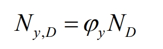
In the formula: 𝑁𝑦, 𝐷 represents the maximum number of uses of the energy storage battery under the condition of the first charge and discharge with a depth of 𝐷; 0 ≤ 𝜑𝑦≤ 1.
The relationship between the depth of charge and discharge of energy storage batteries and their lifespan is obtained through the power function fitting method, as shown in the formula.
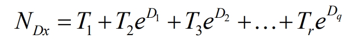
In the formula, 𝑇 1, 𝑇 2, 𝑇 3… 𝑇 𝑟 are the fitting parameters, and 𝐷 1, 𝐷 2, 𝐷 3… are different charging and discharging depths. The curve between the depth of charge and discharge and the service life of battery energy storage systems obtained by fitting laboratory data is shown in Figure 1.
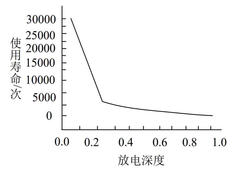
As shown in Figure 1, as the depth of charging and discharging of energy storage batteries increases, their service life decreases, the cost of energy storage battery loss increases, and the economy of microgrids deteriorates. Therefore, during battery energy storage systems operation, the phenomenon of overcharging and discharging of energy storage batteries should be reduced.
3.3 Capacity configuration of battery energy storage system based on improved artificial bee colony algorithm
3.1 Working principle of artificial bee colony algorithm
There are many colony behaviors in nature. For example, when bees are searching for food sources, collecting nectar and exchanging information, they have obvious intelligent behaviors such as division of labor, cooperation and information sharing. The artificial bee colony algorithm (ABC) is a simulation of the process of bees searching for food sources. The earliest artificial bee colony algorithm was proposed by a Türkiye scholar. During the entire algorithm process, bees can be divided into three different types of bee swarms based on the nature of their work: leading bees, following bees, and reconnaissance bees. The mathematical model consists of a food source, a leading bee, and a following bee. The food source represents the feasible solution of the optimization problem in the algorithm and is the main processing object in the algorithm. The leading bee, also known as the hired bee, corresponds to the location of the food source, and the number of food sources is equal to the number of leading bees. The feasible solution for searching optimization problems near the food source is mainly responsible for searching in the neighborhood of the food source, and passing the searched food source location and quantity information to the following bee through a certain probability. Subsequently, the following bee will screen the food based on roulette or greedy selection, Then extract new food sources around the neighborhood. After a certain period of mining, when the leader peak detects food sources and finds that the quality has not improved for multiple generations, they will choose whether to become the investigation peak and continue mining new food sources in the execution area. Similarly, when feasibility solving optimization problems, different food sources will correspond to different solutions of the optimization problem one by one. The quality of any food source is determined by the fitness of the objective function, and the quality of the food source will also increase with the increase of fitness value.
The ABC algorithm is widely used to solve continuous optimization problems due to its weak global and post search capabilities, fewer variables, and the tendency to fall into local optima. It is a new swarm intelligence algorithm proposed to address the cooperative and shared information behavior of bee colonies when searching for food sources. In this algorithm, bees are guided to search for food around the food source neighborhood Following bees will search for food based on the probability calculated using fitness values or roulette wheel bets, and then become reconnaissance bees who will search and discover new food sources
Loop through these three different search methods to find the optimal solution to the problem.
The artificial bee colony algorithm will randomly generate multiple initialization populations in the solution space, assuming each corresponds to a D-dimensional vector, where D is the number of variables in the optimization problem. The position of the i-th food source i ∈ [1, SN] in the D-dimensional vector is defined as Xi ∈ [xi1, xiD].
The initialization formula for the location of the food source is shown in the formula.
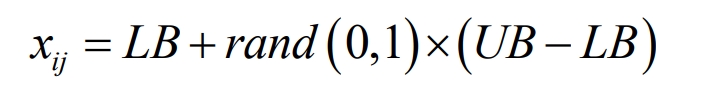
In the formula, 𝑥𝑗 represents the total number of food sources that are randomly generated, 𝑆𝑁 represents the total number of food sources, and 𝑟𝑎𝑛𝑑 (0,1) represents the uniform distribution of random numbers within the range of 0 to 1. 𝐿𝐵 is the optimal solution found, and 𝑈𝐵 is the upper and lower bounds of the components.
Following bees will make food choices based on their judgment of the level of income from food sources. F (ł) is used as the fitness of the food source, and the fitness value is used as the probability evaluation criterion. If F (ł) is higher, the food source will have a greater probability of being selected by the following bee.
The probability formula for selecting food sources is shown in the formula.
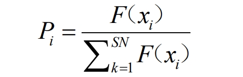
Each food source has a corresponding guide bee, which searches for the location of the food and records and updates the information of the food source. This can be expressed as 𝑉ł=[𝑣ą, 𝑣𝐷], and the search formula is shown in the formula.
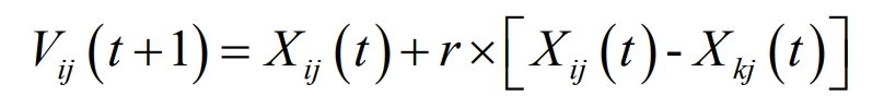
In the formula: Vij is the location of the food source, 𝑗 and 𝑘 are randomly generated and satisfy the conditions i ∈ [1, SN], k ∈ [1, D] and i ≠ k, 𝑟 is any random number, taking random values between (-1, 1). At the same time, following bees will compare the benefits of food sources. If it is found that the benefits of a new food source are better than those of the original food source, the new food source will be chosen, and vice versa, the original food source will be chosen.
After each update, if there is no difference from the previous solution, it indicates that the ABC algorithm has fallen into a local optimal problem, which can indicate that the food source is problematic and should be discarded. At this point, the leading bee acts as a follower bee and continues to search for the location of the food source. At this point, the food source location can be determined using the formula shown in the formula.
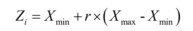
In the formula, 𝑚𝑎𝑥 is the upper boundary of the one-dimensional component, and 𝑚𝑛 is the lower boundary of the one-dimensional component.
The main steps for the corresponding artificial bee colony algorithm to seek the optimal solution are as follows:
Step 1: Firstly, set the relevant parameters of the artificial bee colony algorithm, such as the number of populations, the maximum number of iterations of the algorithm, the maximum search times restricted by the algorithm, and the dimension of the food source;
Step 2: Initialize the food source parameters according to the formula;
Step 3: Each leading bee randomly searches for food sources within its neighborhood, and calculates the corresponding fitness F (ł) value for each food source;
Step 4: Follow the bee to search in the neighborhood of the food source location and further determine the new food source location based on the formula. Afterwards, calculate the fitness F(Xi);
Step 5: Calculate the probability of the food source being selected according to the formula. The following bee will then search in the neighborhood of the food source location, and further determine the new food source location according to the formula. Calculate the fitness of Xi and Vi;
Step 6: After the leader bee reaches the maximum number of searches, the food source remains unchanged and the current food source is abandoned. At this point, the bee transforms into a reconnaissance bee and searches for a new food source according to the formula. If there are no abandoned food sources, proceed to step seven;
Step 7: If the iteration count does not reach the upper limit, proceed to Step 3. If the upper limit is reached, output the optimal food source.
3.2 Improvement of artificial bee colony algorithm
Artificial bee colony algorithm is a very important field of intelligent optimization in recent years. Reference [54] adopts a search strategy of global optimal guidance in the leading bee stage, and the degree of guidance decreases with the number of experiments to balance the global and local search capabilities of ABC algorithm. According to the formula, when the food source is updated, only one dimension is updated at a time. The leader bee can only search within the neighborhood of that dimension without finding any other neighbors. At the same time, the search space will randomly generate multiple feasible solutions distributed within it, resulting in poor accuracy in seeking solutions. This is also one of the main reasons for the low search efficiency of the algorithm. In solving the problem of low efficiency in the ABC algorithm, a comparison mechanism is adopted, which proposes a method of adjusting the number of search dimensions using constant parameters to increase the search neighborhood. After the initialization of the bee colony, when leading the bee to search, it will first generate a random variable with a size between 0 and 1. By comparing the constant parameter with the random variable, it is determined whether the neighborhood search work for this dimension has been carried out. If the generated random variable is greater than the constant parameter, the bee colony starts searching for the neighborhood where the dimension is located. If the generated random variable is less than the constant parameter, the bee colony does not search for the next instruction.
As defined, the larger the dimension, the stronger the search ability of the algorithm. Introducing a dynamic parameter MC (nonlinear value) can improve the local problem of the ABC algorithm. The MC value is shown in the formula:

In the formula, EF represents the number of times the algorithm has converged. This value is a change value, which represents the number of times the algorithm has been evaluated during the convergence process and is a cumulative change value. MaxEFs is the maximum number of iterations set by the ABC algorithm (determined value).
From the above formula, it can be seen that the new food source will slow down the entire algorithm’s search for feasible solutions. In response to the local optimization problem in traditional ABC algorithms, the improvement of ABC algorithms has been studied and discussed by scholars both domestically and internationally. As shown in the formula.
Among them, 𝑟, 𝑘 ∈ {1,2,…, 𝑆 𝑁}, 𝑟 ≠ 𝑘 ≠ Å, j ∈ {1,2,…, D}; 𝑏𝑒𝑠𝑡 represents the globally optimal individual of the population. In equations (3-22) and (3-23), new food sources appear near randomly selected positions, with strong global search ability and poor convergence. Formulas have strong convergence ability, but are prone to local optima.
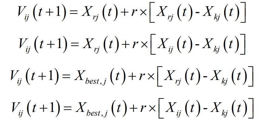
Therefore, the combination of the above five control strategies introduces the idea of coevolution. The new search strategy set is shown in the formula;
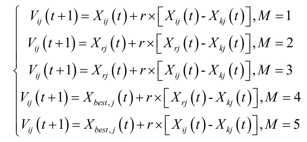
Among them, M=i (mod5)+1 M {1,2,3,4,5}.
The execution steps of the improved ABC algorithm are as follows:
Step 1: Initialize and assign the parameters of the improved ABC algorithm;
Step 2: Calculate the optimal value of each bee colony’s food source;
Step 3: Generate a new food source based on the formula and calculate the corresponding fitness of the food source. By comparing the results through greedy strategies, preserve food sources with higher fitness;
Step 4: Calculate the corresponding selection probability of the food source retained in Step 3 through a formula;
Step 5: After calculating the probability value corresponding to each food source, the following bee will select the optimal value based on the size of the probability value, and then conduct a local search to find new food sources according to the formula;
Step 6: Calculate the objective function value of the new food source found in the previous step, and select the one with higher fitness as the new food source based on the greedy strategy;
Step 7: When the number of iterations of the leading bee reaches the maximum value, its food source position will not change, and this value should be discarded. The leading bee will play the role of a reconnaissance bee, and then continue to generate new food sources according to the formula;
Step 8: Retain the optimal solution and proceed to step 3. When the number of iterations of the improved ABC algorithm reaches the upper limit, output the optimal solution.
3.3 Algorithm testing
In order to verify the optimization effect of the improved ABC algorithm, this article uses four test functions to search for the optimal value of the objective function for the ABC algorithm, GABC algorithm, and the improved ABC algorithm. U represents a unimodal function (with only one maximum value within the interval), M represents a multimodal function (with two or more maximum values within the interval), S represents a separable function (the function library can be decomposed into functions with different functions based on their functions), N represents an inseparable function (the function library cannot be divided into different function functions based on their functions). Represents four types of functions (US unimodal separable function, UN unimodal non separable function, MS multi modal separable function, MN multi modal non separable function), search range, and optimization results.
| Function | Algorithm | Optimal value | Worst value | Average | Standard deviation |
| f1 | ABC | 7.47e-12 | 1.36e-19 | 1.39e-14 | 1.26e-17 |
| f1 | GABC | 7.21e-12 | 1.29e-14 | 8.56e-13 | 1.29e-13 |
| f1 | Improving ABC | 2.14e-104 | 2.24e-105 | 2.57e-104 | 6.14e-105 |
| f2 | ABC | 4.27 | 1.55e1 | 1.11e+1 | 2.33 |
| f2 | GABC | 2.17 | 4.13 | 3.34e | 4.31e-1 |
| f2 | Improving ABC | 5.13e-3 | 2.13e-2 | 1.21e-03 | 5.91e-3 |
| f3 | ABC | 0 | 0 | 0 | 0 |
| f3 | GABC | 0 | 0 | 0 | 0 |
| f3 | Improving ABC | 0 | 6.87 | 2.96 | 1.81 |
| f4 | ABC | 4.45e-1 | 4.77e-1 | 4.67e-1 | 1.11e-2 |
| f4 | GABC | 4.23e-1 | 4.85e-1 | 4.51e-1 | 1.39e-2 |
| f4 | Improving ABC | 8.01e-2 | 1.13e-1 | 1.31e-1 | 1.41e-2 |
During the experiment, set 𝑆𝑁=30, 𝑙𝑚𝑚𝑡=𝑆𝑁 × 𝐷, the maximum number of evaluations for the objective function set in this article is 𝑀𝑎𝑥𝐹𝐸𝑠=5000 × 𝐷. The above ABC algorithm, GABC algorithm, and improved ABC algorithm were simulated and verified 40 times to obtain the optimal results for the test function. MATLAB tests the simulation results of three algorithms with D=60 and D=100, as shown in Tables 1 and 2.
| Function | Algorithm | Optimal value | Worst value | Average | Standard deviation |
| f1 | ABC | 1.78e-15 | 2.43e-15 | 2.31e-15 | 1.24e-16 |
| f1 | GABC | 1.59e-15 | 2.29e-15 | 179e-16 | 1.70e-16 |
| f1 | Improving ABC | 1.72e-107 | 1.81e-104 | 3.28e-106 | 5.32e-105 |
| f2 | ABC | 2.13e1 | 3.13e+01 | 2.59E+01 | 2.29 |
| f2 | GABC | 1.21e+1 | 2.13e+01 | 1.31e+01 | 1.39 |
| f2 | Improving ABC | 1.11 | 3.51 | 2.03 | 6.76e-01 |
| f3 | ABC | 0 | 0 | 0 | 0 |
| f3 | GABC | 0 | 0 | 0 | 0 |
| f3 | Improving ABC | 1.11e1 | 3.45e1 | 2.12e1 | 5.37 |
| f4 | ABC | 4.67e-1 | 4.67e-1 | 4.74e-1 | 1.21e-3 |
| f4 | GABC | 4.53e-1 | 4.61e-1 | 4.74e-1 | 1.29e-3 |
| f4 | Improving ABC | 1.21e-1 | 2.63e-1 | 1.39e-1 | 1.12e-2 |
From Tables 1 and 2, it can be seen that the ABC algorithm, GABC algorithm, and improved ABC algorithm did not achieve optimal values in unimodal functions (𝑓 1 unimodal separable function and 𝑓 2 unimodal non separable function), but the optimal values were relatively stable and more theoretically optimal; Because the three algorithms have a better performance in single peak function optimization compared to ABC algorithm<GABC<improved ABC algorithm, the improved ABC algorithm is better under the single peak function optimization ability. The ABC algorithm, GABC algorithm, and improved ABC algorithm did not achieve ideal optimization results in the process of finding the optimal value of multimodal functions (𝑓 3 multimodal separable functions and 𝑓 4 multimodal nonseparable functions), especially when the 𝑓 3 multimodal separable function did not find the ideal optimal value, and both ABC algorithm and GABC algorithm found the ideal optimal value, which can be expressed as ABC algorithm=GABC algorithm=improved ABC algorithm, Because the principle of using dynamic parameters to improve the ABC algorithm is similar to the differential evolution method, the differential evolution method cannot find the optimal solution for 𝑓 3 multi peak differentiable functions; 𝑓 4 Multi peak indivisible function is a complex nonlinear multi-objective function that is prone to falling into local optima when solved by algorithms. Compared with ABC algorithm and GABC algorithm, the improved ABC algorithm improves the particle search ability, and the optimization effect is that ABC algorithm ≈ GABC algorithm<improved ABC algorithm.
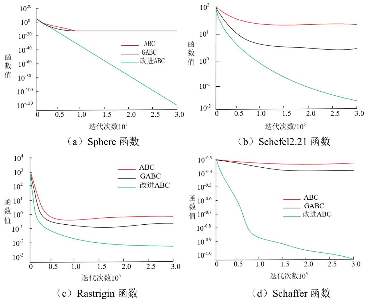
Figure 2 shows the convergence of the ABC algorithm, GABC algorithm, and improved ABC algorithm in four test functions: 𝑓 1 unimodal separable function, 𝑓 2 unimodal indivisible function, 𝑓 3 multi modal separable function, and 𝑓 4 multi modal indivisible function. Under the conditions of 𝑓 1 single peak separable function and 𝑓 2 single peak non separable function, the improved ABC algorithm decreases in a straight line form, while the ABC algorithm and GABC algorithm have almost no change in function values when the number of iterations is 10 ^ 5. In 𝑓 3, although the improved ABC algorithm does not decrease in a straight line form, the convergence effect of the improved ABC algorithm is better compared to the ABC algorithm and the improved ABC algorithm. For 𝑓 4 multi peak indivisible functions, using algorithms to solve them can easily fall into local optima, but using dynamic parameter improvement ABC algorithm to increase particle search ability is more likely to improve particle search ability and improve optimization results.
4. Simulation results and analysis
| Unit type | Capacity (kW) | Fuel cost (yuan/kWh) | Maintenance cost (yuan/kWh) | Forced outage rate (%) | Quantity (set) |
| Internal combustion engine | 800 | 0.72 | 0.01 | 5.2 | 3 |
| Micro gas turbine | 800 | 0,90 | 0.12 | 0.5 | 2 |
| Fuel cell | 200 | 0.58 | 0.31 | 0.5 | 1 |
| Total | 4200 | — | — | — | 6 |
Configure the capacity of the island operating microgrid battery energy storage systems based on the improved ABC algorithm. The maximum power load for this example is 4100kW, and in principle, 5 800kW generators and 1 200kW engine are required. The specific parameters are shown in Table 3. The parameters of lithium-ion batteries in battery energy storage systems are shown in Table 4, and the time-of-use electricity price table for microgrids is shown in Table 5.
| lithium battery | |
| Energy storage life (times) | 3000 |
| Charging and discharging efficiency (%) | 90 |
| Unit price of capacity (yuan/Wh) | 1 |
| Maintenance unit price (yuan/Wh) | 0.05 |
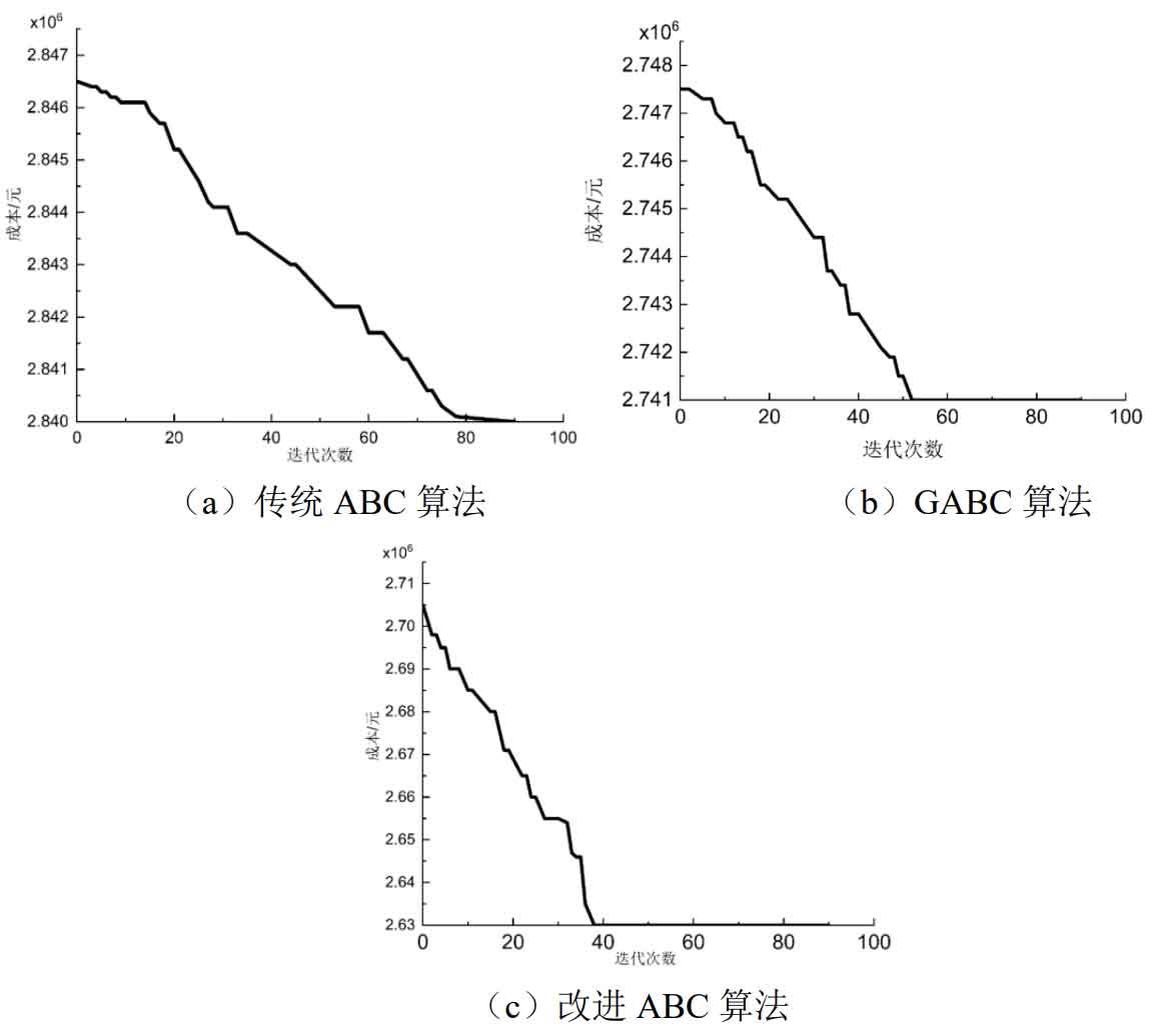
For the established optimization model, the traditional ABC algorithm, GABC algorithm, and the improved ABC algorithm proposed in this article were used to configure the capacity of the island operating microgrid in this example. The iterative solution process of the three algorithms is shown in Figure 3, and the final battery energy storage systems capacity optimization configuration results are shown in Table 5.
| Time period (h) | Electricity price (yuan/kWh) |
| Peak period (9-12,17-21) | 1.1113 |
| Valley period (0-5,22-23) | 0.6113 |
| Normal period (6-8, 13-16) | 0.8113 |
From the data in Figure 3 and Table 5, it can be seen that the capacity configuration using ENNS in the random simulation production method does not meet the load shortage rate 𝑓𝐿, and in this case, the capacity configuration is omitted. The load shortage rate of LOLP, traditional ABC algorithm, GABC algorithm, and improved ABC algorithm in the random simulation production method for battery energy storage systems capacity configuration meets the requirements. The battery energy storage systems capacity configured by LOLP in the random simulation production method is 1100 kWh, with a cost of 2.925 million yuan and a load shortage rate of 0.210; When using the traditional ABC algorithm configuration, the battery energy storage systems capacity is 1000kWh, the cost is 2.840 million yuan, the number of iterations is 80, and the load shortage rate is 0.2235; When using GABC algorithm to optimize the capacity configuration of battery energy storage systems, the capacity is 950kWh, the cost is 2.748 million yuan, the number of iterations is 52, and the load shortage rate is 0.2341; The improved ABC algorithm in this article optimizes the capacity configuration of battery energy storage systems with a capacity of 900kWh, a cost of 2.63 million yuan, 40 iterations, and a load outage probability of 0.2341.
From this, it can be seen that under the condition of meeting the load shortage rate, the cost ranking of microgrids is: random simulation production method>traditional ABC algorithm>GABC algorithm>improved ABC algorithm. The simulation results show that the improved artificial bee colony algorithm achieves capacity allocation by solving the objective function, which increases the economic efficiency of the microgrid by 10% compared to the random production simulation method.
| Optimize parameters | LOLP | ENNS | Traditional ABC algorithm | GABC algorithm | Improved ABC algorithm |
| Load shortage rate fL | 0210 | 0.35 | 0.2235 | 0.2341 | 0.2471 |
| Energy loss rate fel | 0.043 | 0.042 | 0.043 | 0.044 | 0.045 |
| Battery capacity/kWh | 1100 | 750 | 1000 | 950 | 900 |
| Cost/million yuan | 2.925 | 2.420 | 2.840 | 2.741 | 2.630 |
| Iterations/time | 0 | 0 | 80 | 52 | 40 |
The improved ABC algorithm is used to configure the capacity of battery energy storage systems, and the battery capacity is 900kWh. Compared to the distributed energy storage of battery energy storage systems, the centralized energy storage control strategy of battery energy storage systems is simpler and easier to operate, so the centralized battery energy storage systems voltage control strategy is adopted.
Firstly, the shortcomings of the random production simulation method for capacity allocation were introduced, and an intelligent algorithm was proposed for capacity allocation of battery energy storage systems. A capacity optimization configuration model for island operating battery energy storage systems has been established, with battery energy storage systems charging and discharging SOC, load shortage rate, charging and discharging constraints, and battery energy storage systems lifespan model as constraints. The traditional ABC algorithm has the problem of local optimal solution in the solving process, introducing dynamic parameters to increase the dimensions of the bee colony in searching for food, increasing the early global and late local search. Using test functions to validate the ABC algorithm, GABC algorithm, and improved ABC algorithm, the validation results show that the improved ABC algorithm is the best. The improved ABC algorithm is applied to solve the capacity optimization configuration model of battery energy storage systems in island operating microgrid systems. Compared with the random production simulation method, traditional ABC algorithm, and GABC algorithm for capacity configuration, the cost of microgrid is the lowest, and compared with the traditional random production simulation method for capacity configuration, the economic efficiency of microgrid is improved by 10%. The improved ABC algorithm for capacity allocation has been validated to ensure the reliability of microgrid power supply, and the battery energy storage systems capacity allocation obtained by the proposed improved ABC algorithm has better economic benefits.