
We propose a comprehensive evaluation framework for battery energy storage systems that integrates technical, economic, and environmental criteria under wind–photovoltaic–battery synergy. By employing fuzzy analytic hierarchy process (FAHP) to derive weights, we establish an optimization model for hourly charging/discharging power allocation. A hybrid grey wolf optimizer with Lévy flight (LF-GWO) is developed to solve the model. Case studies based on meteorological and load data from a region in Xinjiang compare five battery energy storage systems: lithium-ion, lithium iron phosphate (LFP), sodium-sulfur (NaS), vanadium redox flow (VRB), and supercapacitor storage (SCSS). The results demonstrate the superiority of the proposed method and provide guidance for selecting battery energy storage systems and optimizing their operation strategies.
1. Introduction
Modern power systems are transitioning toward high shares of renewable energy sources. The inherent variability and uncertainty of wind and solar power require flexible resources to maintain balance. battery energy storage systems, with their bidirectional power capability and fast response, are key enablers for peak shaving, frequency regulation, and renewable energy integration. However, selecting the appropriate battery energy storage system involves multiple conflicting objectives: cost, efficiency, lifetime, environmental impact, and operational benefits. Existing studies often focus on a single aspect, such as economics or technical performance, lacking a holistic perspective. We address this gap by developing a comprehensive evaluation system that captures the whole life cycle of battery energy storage systems under wind–photovoltaic–battery synergy. Our approach systematically quantifies economic, technical, and environmental indices and optimizes the charging/discharging strategy to maximize overall benefit.
2. Whole-Life-Cycle Benefit Model of Battery Energy Storage Systems
The total economic benefit of a battery energy storage system over its lifetime is expressed as the sum of investment cost, operation and maintenance cost, revenue from arbitrage and avoided wheeling charges, government subsidies, and the value of deferred grid upgrade. The environmental benefit is measured by the reduction in carbon emissions when the battery energy storage system is coordinated with wind and photovoltaic generation. Technical indices include lifetime efficiency, state-of-charge limits, and peak-shaving capability.
2.1 Economic Model
The net economic value is given by:
$$
C_{\mathrm{eco}} = C_{\mathrm{inv}} + C_{\mathrm{op}} – C_{\mathrm{pro}} – C_{\mathrm{sub}}
$$
where \(C_{\mathrm{inv}}\) is the annualized investment cost, \(C_{\mathrm{op}}\) the operation and maintenance cost, \(C_{\mathrm{pro}}\) the revenue, and \(C_{\mathrm{sub}}\) the subsidy income. The investment cost is converted to an annuity using the discount rate \(r\) and battery lifetime \(y_b\):
$$
C_{\mathrm{inv}} = \frac{r(1+r)^{y_b}}{(1+r)^{y_b}-1} \left( C_p \bar{P} + C_e E_N \right)
$$
Here \(C_p\) is the power-related cost per kW, \(\bar{P}\) the absolute charging/discharging power, \(C_e\) the energy-related cost per kWh, and \(E_N\) the rated capacity. Operation cost includes maintenance and the benefit from deferring grid upgrade:
$$
C_{\mathrm{op}} = C_{\mathrm{main}} – C_{\mathrm{upgrade}}
$$
The annual maintenance cost is proportional to absolute power:
$$
C_{\mathrm{main}} = \sum_{t=1}^{24} C_m P_{\mathrm{ESS}}(t) \, y_b
$$
The deferral period \(\Delta n\) depends on the load growth rate \(\tau\) and the peak-shaving ratio \(\lambda\):
$$
\lambda = 1 – \frac{\min(P_{\mathrm{load}}(t) – P_{\mathrm{cd}}(t))}{\max(P_{\mathrm{load}}(t) – P_{\mathrm{cd}}(t))}, \quad \Delta n = \frac{\lg(1+\lambda)}{\lg(1+\tau)}
$$
where \(P_{\mathrm{cd}}(t) = P_{\mathrm{dis}}(t)U_{\mathrm{dis}}(t) – P_{\mathrm{cha}}(t)U_{\mathrm{cha}}(t)\) with binary variables satisfying \(U_{\mathrm{dis}}(t)+U_{\mathrm{cha}}(t)=1\) and \(U_{\mathrm{dis}}(t)\cdot U_{\mathrm{cha}}(t)=0\). The upgrade deferral benefit is calculated as:
$$
C_{\mathrm{upgrade}} = C_w \left| 1 – \frac{r(1+r)^{\Delta n}}{(1+r)^{\Delta n}-1} \right|
$$
Revenue comes from energy arbitrage and avoided wheeling charges:
$$
C_{\mathrm{pro}} = C_{\mathrm{LSHI}} + C_{\mathrm{ESF}}
$$
The daily arbitrage profit is:
$$
C_{\mathrm{LSHI,per}} = \sum_{t=1}^{24} P_{\mathrm{cd}}(t) c_{\mathrm{pric}}(t)
$$
and over the lifetime using average annual operating days \(D\):
$$
C_{\mathrm{LSHI}} = C_{\mathrm{LSHI,per}} \cdot y_b \cdot D
$$
The avoided wheeling cost is:
$$
C_{\mathrm{ESF}} = \sum_{t=1}^{24} D \cdot (P_{\mathrm{dis}}(t)-P_{\mathrm{cha}}(t)) \, c_r(t) \, y_b, \quad c_r(t) = \rho c_{\mathrm{pric}}(t)
$$
Government subsidy is:
$$
C_{\mathrm{sub}} = D \cdot \sum_{t=1}^{24} P_{\mathrm{dis}}(t)U_{\mathrm{dis}}(t) \, c_{\mathrm{sub}} \, y_b
$$
Carbon emissions from conventional generation are:
$$
C_{\mathrm{emi}} = \sum_{t=1}^{24} D \cdot P_g(t) \cdot e_{\mathrm{carbon}} \cdot y_b
$$
$$
P_g(t) = P_{\mathrm{load}}(t) – P_{\mathrm{PV}}(t) – P_{\mathrm{WT}}(t) – P_{\mathrm{cd}}(t)
$$
We set \(e_{\mathrm{carbon}} = 0.636\) kg CO\(_2\)/kWh.
3. Fuzzy Analytic Hierarchy Process for Comprehensive Evaluation
FAHP extends the traditional AHP by using fuzzy complementary matrices to handle uncertainty in pairwise comparisons. The hierarchy consists of a goal layer (overall benefit), a criterion layer (environmental, economic, technical), an indicator layer (11 specific metrics), and a decision layer (five candidate battery energy storage systems).
3.1 Fuzzy Complementary Matrix and Consistency
A fuzzy matrix \(S = (s_{ij})_{n\times n}\) is complementary if \(s_{ij}+s_{ji}=1\) and \(s_{ii}=0.5\). When the matrix also satisfies \(s_{ij}=s_{ik}-s_{jk}+0.5\) for all \(i,j,k\), it is a fuzzy consistent matrix. The conversion from a fuzzy complementary matrix to a consistent one uses:
$$
s_{ij} = \frac{\sum_{k=1}^n s_{ik} – \sum_{k=1}^n s_{jk}}{2n} + 0.5
$$
3.2 Weight Calculation
The weight of criterion \(R_i\) with respect to goal \(F_k\) is:
$$
\omega_i^k = \frac{2\alpha – n + 2\sum_{j=1}^n s_{ij}}{2n\alpha}, \quad \alpha \ge \frac{n-1}{2}
$$
The global weight of indicator \(T_i\) is:
$$
T_i = \sum_{k=1}^n \mu_k \omega_i^k
$$
where \(\mu_k\) is the weight of indicator under criterion \(R_i\).
3.3 Hierarchy Structure
We define the goal as “Optimal selection of battery energy storage system”. The criteria are: Environmental (S1), Economic (S2), Technical (S3). Indicators include: carbon emission (T1), investment cost (T2), O&M cost (T3), arbitrage revenue (T4), avoided wheeling (T5), subsidy (T6), deferral benefit (T7), lifetime (T8), efficiency (T9), SOC range (T10), peak-shaving ratio (T11). The decision layer contains five types of battery energy storage systems. The pairwise comparison matrices are constructed using the scale in Table 1.
| Scale | Definition | Explanation |
|---|---|---|
| 0.5 | Equal importance | Element i and j are equally important |
| 0.6 | Slightly more important | Element i is slightly more important than j |
| 0.7 | Clearly more important | Element i is clearly more important than j |
| 0.8 | Much more important | Element i is much more important than j |
| 0.9 | Extremely more important | Element i is extremely more important than j |
| 0.1–0.4 | Reverse comparison | Opposite of the above |
3.4 Priority Matrices
| S1 | S2 | S3 | |
|---|---|---|---|
| S1 | 0.5 | 0.7 | 0.8 |
| S2 | 0.3 | 0.5 | 0.6 |
| S3 | 0.2 | 0.4 | 0.5 |
| T2 | T3 | T4 | T5 | T6 | T7 | |
|---|---|---|---|---|---|---|
| T2 | 0.5 | 0.5 | 0.7 | 0.6 | 0.3 | 0.4 |
| T3 | 0.5 | 0.5 | 0.7 | 0.6 | 0.3 | 0.4 |
| T4 | 0.3 | 0.3 | 0.5 | 0.4 | 0.1 | 0.2 |
| T5 | 0.4 | 0.4 | 0.6 | 0.5 | 0.2 | 0.3 |
| T6 | 0.7 | 0.7 | 0.9 | 0.8 | 0.5 | 0.6 |
| T7 | 0.6 | 0.6 | 0.8 | 0.7 | 0.4 | 0.5 |
| T8 | T9 | T10 | T11 | |
|---|---|---|---|---|
| T8 | 0.5 | 0.4 | 0.4 | 0.3 |
| T9 | 0.6 | 0.5 | 0.5 | 0.4 |
| T10 | 0.6 | 0.5 | 0.5 | 0.4 |
| T11 | 0.7 | 0.6 | 0.6 | 0.5 |
After converting to fuzzy consistent matrices and computing weights, we obtain: environmental weight 0.2167, economic weight 0.3667, technical weight 0.4166. Among economic indicators, arbitrage revenue receives the highest weight (20.66%); among technical indicators, lifetime receives the highest weight (28.33%).
4. Optimization Model for battery energy storage system under Wind-Photovoltaic-Battery Synergy
4.1 Wind Turbine Model
The hourly power output of a wind turbine depends on wind speed:
$$
P_{\mathrm{WT}}(t) = \begin{cases}
0, & vv_o \\
\eta_{\mathrm{WT}} P_{\mathrm{rated}}^{\mathrm{WT}} \frac{v^3(t)-v_i^3}{v_r^3-v_i^3}, & v_i \le v \le v_r \\
\eta_{\mathrm{WT}} P_{\mathrm{rated}}^{\mathrm{WT}}, & v_r \le v \le v_o
\end{cases}
$$
Wind speed at hub height is adjusted from measured data:
$$
v(t) = v_{\mathrm{ref}}(t) \frac{\ln(h/z_0)}{\ln(h_{\mathrm{ref}}/z_0)}
$$
4.2 Photovoltaic Model
The PV output power is:
$$
P_{\mathrm{PV}}(t) = \eta_{\mathrm{STC}}^{\mathrm{PV}} \left[ \frac{9.5 \mu_{\mathrm{PV}} (T_{\mathrm{NOCT}}-20)(1-\eta_{\mathrm{STC}}^{\mathrm{PV}})}{800 \eta_{\mathrm{STC}}^{\mathrm{PV}} (5.7+3.8v(t))} G_g(t) + \left( \frac{\mu_{\mathrm{PV}}}{\eta_{\mathrm{STC}}^{\mathrm{PV}}}(T(t)-T_{\mathrm{STC}})+1 \right) \right] G_g(t) A_{\mathrm{PV}}
$$
4.3 Objective Function
The goal is to minimize the weighted sum of environmental, economic, and technical costs:
$$
\min F = \omega_1 C_{\mathrm{emi}} + \omega_2 C_{\mathrm{eco}} + \omega_3 C_{\mathrm{tec}}
$$
where
$$
\begin{aligned}
C_{\mathrm{eco}} &= \mu_1 C_{\mathrm{inv}} + \mu_2 C_{\mathrm{main}} – \mu_3 C_{\mathrm{LSHI}} – \mu_4 C_{\mathrm{ESF}} – \mu_5 C_{\mathrm{sub}} – \mu_6 C_{\mathrm{upgrade}}, \\
C_{\mathrm{tec}} &= \mu_1 y_b + \mu_8 \eta_{\mathrm{ESS}} + \mu_9 \theta + \mu_{10} \lambda
\end{aligned}
$$
\(\theta\) represents SOC range; \(\lambda\) peak-shaving ratio.
4.4 Constraints
battery energy storage system constraints:
$$
\begin{aligned}
\sum_{t=1}^{24} P_{\mathrm{cha}}(t) &\le E_N, \\
S_{\min} &\le S(t) \le S_{\max}, \\
\sum_{t=1}^{24} (P_{\mathrm{dis}}(t) – P_{\mathrm{cha}}(t)\eta_{\mathrm{ESS}}) &= 0, \\
E_{\min} &\le E_N \le E_{\max}
\end{aligned}
$$
Photovoltaic and wind constraints:
$$
0 \le P_{\mathrm{PV}}(t) \le P_{\max}^{\mathrm{PV}}, \quad 0 \le P_{\mathrm{WT}}(t) \le P_{\max}^{\mathrm{WT}}
$$
5. LF-GWO Hybrid Optimization Algorithm
The standard grey wolf optimizer (GWO) suffers from slow convergence and local optima. We enhance it with Circle chaotic initialization, adaptive nonlinear convergence factor, adaptive inertia weight, and Lévy flight (LF) strategy. The improved algorithm is called LF-GWO.
5.1 Circle Chaotic Map
Initial population diversity is improved via:
$$
X_i = \bmod\left( X_i + 0.2 – \frac{0.5}{2\pi} \sin(2\pi X_i), 1 \right)
$$
5.2 Nonlinear Convergence Factor
The linear decreasing \(a\) is replaced by:
$$
a = (a_{\mathrm{initial}} – a_{\mathrm{final}}) \left( 1 – \frac{i}{M} \right)^2
$$
where \(M\) is maximum iterations.
5.3 Adaptive Inertia Weight
We use a cosine-based adaptive weight:
$$
J = h \cdot \cos\left( \frac{\pi}{2} \sin\left( \frac{i}{M} \right) \right)
$$
with \(h=0.2\). The position update becomes:
$$
X_{\mathrm{pos}}^{i+1} = \frac{1}{3} \sum_{n=\alpha,\beta,\delta} (J \cdot X_n^i – A_n D_n)
$$
5.4 Lévy Flight Strategy
When the algorithm is trapped in local optima, a Lévy flight is applied:
$$
X_{\mathrm{pos}}^{i+1} = X_{\mathrm{pos}}^i + \xi \oplus L(\beta)
$$
where \(\xi\) is a random number in [0,1] and \(L(\beta)\) follows the Lévy distribution with parameter \(\beta=1.5\). The step is generated via Mantegna’s algorithm:
$$
s = \frac{u}{|v|^{1/\beta}}, \quad u \sim N(0,\sigma^2), \quad v \sim N(0,1), \quad \sigma = \left[ \frac{\Gamma(1+\beta)\sin(\pi\beta/2)}{\Gamma((1+\beta)/2) \cdot 2^{(\beta-1)/2}} \right]^{1/\beta}
$$
5.5 Algorithm Validation
We compared LF-GWO with standard GWO and PSO on benchmark functions (Sphere, Schwefel, Rastrigin, Ackley, Shekel’s Foxholes, Goldstein-Price). Results are shown in Table 5.
| Function | Metric | PSO | GWO | LF-GWO |
|---|---|---|---|---|
| f1 (Sphere) | Ave | 2.37e-5 | 3.72e-27 | 0.00e0 |
| Std | 2.52e-5 | 4.67e-27 | 0.00e0 | |
| f2 (Schwefel) | Ave | 6.60e-3 | 4.53e-17 | 0.00e0 |
| Std | 2.58e-3 | 7.81e-17 | 0.00e0 | |
| f9 (Rastrigin) | Ave | 1.32e2 | 1.14e-13 | 0.00e0 |
| Std | 1.76e2 | 4.30e-13 | 0.00e0 | |
| f10 (Ackley) | Ave | 2.52e1 | 1.11e-14 | 8.88e-16 |
| Std | 8.60e1 | 4.08e-14 | 2.25e-16 | |
| f14 (Shekel) | Ave | 6.90e0 | 2.98e0 | 1.27e1 |
| Std | 2.64e0 | 8.01e0 | 3.22e1 | |
| f18 (Goldstein-Price) | Ave | 3.00e0 | 3.00e0 | 3.00e0 |
| Std | 3.96e-6 | 7.85e-6 | 1.93e-6 |
LF-GWO reaches the global optimum for unimodal and many multimodal functions with faster convergence. It also escapes local optima effectively.
6. Case Study
6.1 Data and Parameters
We use hourly meteorological data (wind speed, temperature, solar irradiance) for a region in Xinjiang in 2022. Wind turbine and photovoltaic parameters are listed in Table 6.
| Component | Parameter | Value |
|---|---|---|
| WT | Efficiency \(\eta_{\mathrm{WT}}\) | 47% |
| Surface roughness \(z_0\) | 15 m | |
| Cut-in speed \(v_i\) | 2.5 m/s | |
| Rated speed \(v_r\) | 8 m/s | |
| Cut-out speed \(v_o\) | 25 m/s | |
| Rated power \(P_{\mathrm{rated}}^{\mathrm{WT}}\) | 1.5 MW | |
| Hub height \(h\) | 70 m | |
| PV | Efficiency at STC \(\eta_{\mathrm{STC}}^{\mathrm{PV}}\) | 17% |
| Temperature coefficient \(\mu_{\mathrm{PV}}\) | -0.32%/°C | |
| STC temperature \(T_{\mathrm{STC}}\) | 25°C | |
| NOCT \(T_{\mathrm{NOCT}}\) | 45°C | |
| Max power \(P_{\max}^{\mathrm{PV}}\) | 330 W | |
| Module area \(A_{\mathrm{PV}}\) | 3 m² |
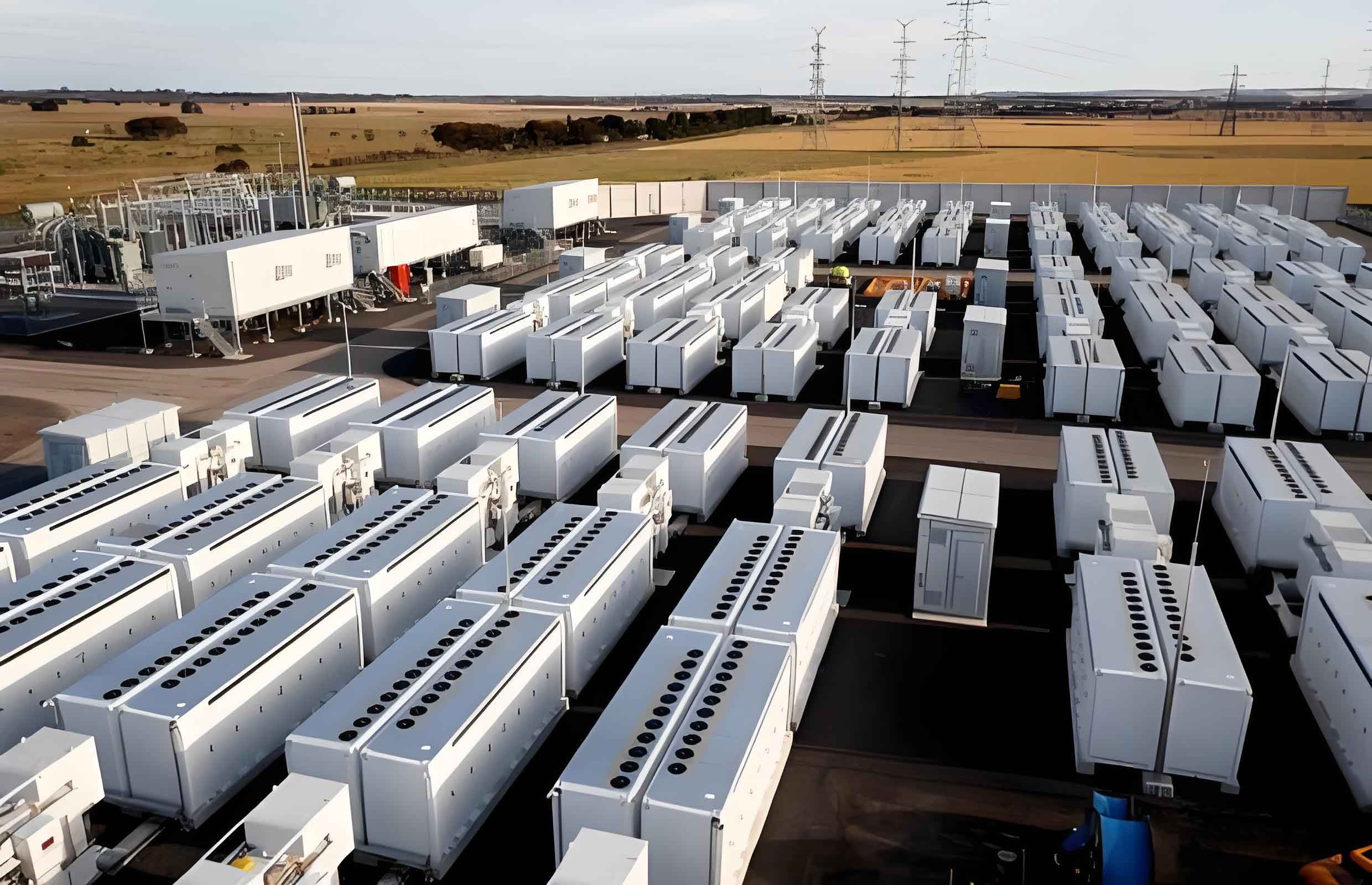
The time-of-use electricity price is shown in Table 7. The average daily load curve and price schedule are illustrated in the following figure (we include a representative image of a battery energy storage system).
| Period | Time interval | Price (yuan/kWh) |
|---|---|---|
| Valley | 00:00–08:00 | 0.13 |
| Flat | 08:00–11:00, 15:00–19:00, 22:00–00:00 | 0.38 |
| Peak | 11:00–15:00, 19:00–22:00 | 0.65 |
Parameters for the five candidate battery energy storage systems are given in Table 8.
| Parameter | Li-ion | LFP | NaS | VRB | SCSS |
|---|---|---|---|---|---|
| \(C_p\) (yuan/kW) | 2950 | 1100 | 1650 | 2940 | 1380 |
| \(C_e\) (yuan/kWh) | 1450 | 880 | 1270 | 690 | 2070 |
| \(C_m\) (yuan/kWh) | 0.1890 | 0.1512 | 0.1701 | 0.1701 | 0.1701 |
| \(\eta_{\mathrm{ESS}}\) (%) | 90 | 70 | 80 | 70 | 95 |
| \(y_b\) (years) | 15 | 8 | 15 | 15 | 20 |
| \(\xi\) (depth of discharge factor) | 0.8 | 0.7 | 0.6 | 0.6 | 0.9 |
| \([S_{\min}, S_{\max}]\) (%) | [20,80] | [30,70] | [10,90] | [20,80] | [10,90] |
6.2 FAHP Weights
From the fuzzy consistent matrices, the computed weights are: environmental 0.2167, economic 0.3667, technical 0.4166. Among economic indicators, arbitrage revenue carries 20.66% weight; among technical indicators, lifetime carries 28.33%.
6.3 Optimization Results
We apply the LF-GWO algorithm to determine the optimal hourly charging/discharging power for each battery energy storage system. The population size is 30, maximum iterations 100. Figure 9 (in the original paper) shows the SOC and power profiles for the five systems. Here we summarize the key economic, environmental, and technical outcomes.
6.4 Economic Comparison
Table 9 lists the breakdown of costs and benefits for each battery energy storage system over its whole life cycle.
| Indicator | Li-ion | LFP | NaS | VRB | SCSS |
|---|---|---|---|---|---|
| Investment cost | 5.2 | 3.1 | 3.8 | 2.9 | 4.5 |
| O&M cost | 1.8 | 0.9 | 1.2 | 1.0 | 2.1 |
| Arbitrage revenue | 3.4 | 2.0 | 3.1 | 3.3 | 4.8 |
| Wheeling saving | 0.6 | 0.3 | 0.5 | 0.5 | 0.9 |
| Subsidy | 0.2 | 0.1 | 0.2 | 0.2 | 0.3 |
| Deferral benefit | 0.8 | 0.4 | 0.7 | 0.6 | 1.0 |
| Net benefit | 1.0 | -0.4 | 1.5 | 2.1 | 2.6 |
SCSS yields the highest net benefit, followed by VRB. LFP has a negative net benefit due to short lifetime and lower efficiency.
6.5 Environmental Comparison
Figure 11 in the original paper shows the CO₂ emission reduction. We present the numerical values in Table 10.
| System | Li-ion | LFP | NaS | VRB | SCSS |
|---|---|---|---|---|---|
| Reduction | 6563 | 4612 | 6731 | 6910 | 11465 |
SCSS achieves the greatest emission reduction due to its longest lifetime and highest efficiency. LFP shows the smallest reduction.
6.6 Technical Comparison
We compute a comprehensive technical score by weighting lifetime, efficiency, SOC range, and peak-shaving ratio. The scores are normalized to a scale of 0–25. Results are in Table 11.
| System | Li-ion | LFP | NaS | VRB | SCSS |
|---|---|---|---|---|---|
| Score | 18.2 | 12.5 | 17.8 | 16.4 | 22.1 |
SCSS ranks highest, followed by Li-ion and NaS. LFP performs worst due to lower efficiency and shorter lifetime.
6.7 Overall Benefit and Selection
Combining the three dimensions with FAHP weights, the overall benefit for each battery energy storage system is computed. SCSS emerges as the best choice when the system can afford the initial investment. For smaller distribution networks with limited budget, NaS or VRB offer a good balance between cost and performance. Li-ion remains a mature technology but with higher cost. LFP is not recommended due to poor economic and technical performance.
7. Conclusion
We have developed a comprehensive evaluation and selection framework for battery energy storage systems under wind–photovoltaic–battery synergy. The main contributions are:
- Establishment of a whole-life-cycle benefit model covering economic, environmental, and technical aspects.
- Application of FAHP to determine the weights of multiple indicators, avoiding inconsistency in traditional AHP.
- An optimization model that minimizes a weighted objective function to find the optimal charging/discharging strategy.
- A novel hybrid LF-GWO algorithm that outperforms standard GWO and PSO in convergence speed and global search ability.
Case studies comparing five battery energy storage systems show that SCSS provides the highest net benefit and greatest emission reduction, but requires higher upfront cost. NaS and VRB are suitable alternatives for cost-sensitive applications. The proposed methodology offers valuable guidance for selecting and operating battery energy storage systems in future power systems.