
The large-scale integration of renewable energy sources, primarily through power electronic converters, is fundamental to the global energy transition. The grid-connected inverter serves as the critical interface, responsible for converting DC power from sources like photovoltaics and wind turbines into grid-compliant AC power. A cornerstone of its operation is maintaining stable synchronization with the utility grid, typically achieved via a Phase-Locked Loop (PLL). Under normal grid conditions, this synchronization is robust. However, during grid faults, the system experiences significant disturbances. Grid codes worldwide mandate that renewable generation plants must possess Low Voltage Ride-Through (LVRT) capability, meaning they must remain connected and support the grid during voltage sags by injecting reactive current. This mandatory operational shift fundamentally alters the output state of the grid-connected inverter. In weak grid scenarios characterized by non-negligible grid impedance, the interaction between the inverter’s control (especially the PLL) and the grid network is intensified. This interaction can destabilize the synchronization mechanism, leading to loss of synchronism (失步) during or after the fault. While existing research has explored aspects of small-signal stability and control design for LVRT, a unified framework that quantitatively assesses the existence of a stable operating point and comprehensively analyzes both transient and small-signal stability margins is lacking. This gap makes it difficult to accurately evaluate and ensure the synchronous operation capability of a grid-connected inverter throughout the entire LVRT event.
This article delves into the synchronous stability of grid-connected inverters during LVRT operation from a holistic perspective. We begin by establishing a nonlinear model that incorporates the LVRT characteristics. A key focus is the quantitative analysis of the Quasi-Static Equilibrium Point (QSEP)—the post-fault steady-state operating point where synchronization is theoretically possible. We derive explicit existence conditions for this QSEP, moving beyond qualitative descriptions. Subsequently, we dissect the synchronization mechanism by separately examining the transient synchronization stability (the ability to reach the QSEP after a large disturbance) and the small-signal stability (the ability to maintain stable operation near the QSEP). This analysis reveals that during grid faults, a grid-connected inverter faces a dual threat: risk of transient loss of synchronism and a degraded small-signal stability margin at the new operating point. To address these challenges, we propose a novel optimization strategy based on the adaptive adjustment of PLL parameters. This strategy dynamically modifies the PLL’s integral gain in response to the grid state, effectively enhancing both the transient stability margin and the small-signal damping of the system, without requiring precise knowledge of grid parameters. Finally, the correctness of the theoretical analysis and the effectiveness of the proposed strategy are validated through detailed time-domain simulations and experimental results.
System Modeling and LVRT Characteristics
The topology and standard control structure of a three-phase grid-connected inverter system are considered. The core synchronization unit is the PLL, which typically uses a Proportional-Integral (PI) controller to regulate the quadrature-axis voltage ($V_q$) to zero, thereby aligning the controller’s reference frame with the grid voltage vector. The dynamic response of the current control loop is significantly faster than that of the PLL. Therefore, for stability analysis focusing on synchronization, the current loop can be reasonably approximated as a static gain, i.e., $I_d = I_{dref}$ and $I_q = I_{qref}$. This simplification allows us to concentrate on the nonlinear interaction between the PLL and the grid.
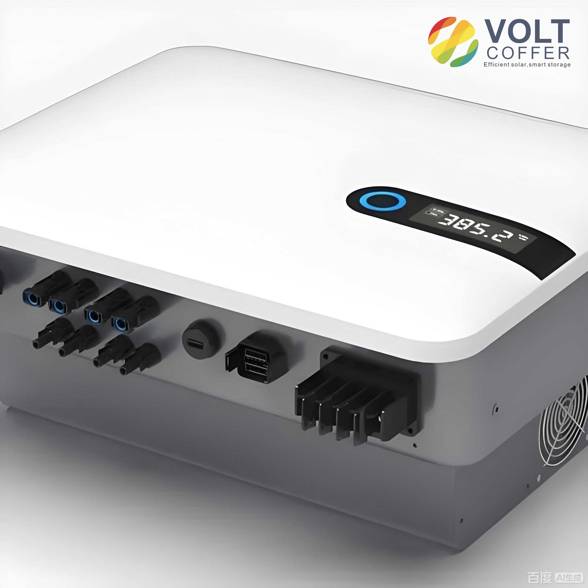
The fundamental synchronization dynamics of the grid-connected inverter are governed by the PLL and the network equations. The PLL dynamics can be described by:
$$\omega_{pll} = \omega_0 + \left(K_p + \frac{K_i}{s}\right) V_q, \quad \theta_{pll} = \int \omega_{pll} dt$$
where $\omega_{pll}$ and $\theta_{pll}$ are the PLL’s estimated frequency and angle, $\omega_0$ is the nominal grid frequency, and $K_p$, $K_i$ are the PI controller gains. Defining the power angle $\delta$ as the angle difference between the PLL reference frame and the actual grid voltage vector ($\delta = \theta_{pll} – \theta_g$), its derivative is:
$$\frac{d\delta}{dt} = \omega_{pll} – \omega_g = \Delta\omega$$
The voltages $V_d$ and $V_q$ at the Point of Common Coupling (PCC) are functions of the grid voltage, grid impedance, output currents, and the power angle:
$$
\begin{aligned}
V_d &= V_g \cos\delta + R_g I_d – X_g I_q \\
V_q &= -V_g \sin\delta + R_g I_q + X_g I_d
\end{aligned}
$$
where $V_g$ is the grid voltage magnitude, and $R_g + jX_g$ is the grid impedance ($X_g = \omega_g L_g$).
During an LVRT event, grid codes require the grid-connected inverter to provide reactive current support. A typical LVRT characteristic is defined as:
$$
I_q = \begin{cases}
-K(0.9 – V_{pcc}), & \text{if } K(0.9 – V_{pcc}) \leq I_{max} \\
-I_{max}, & \text{if } K(0.9 – V_{pcc}) > I_{max}
\end{cases}
$$
where $K$ is the reactive current gain (usually between 1.5 and 2.5 per unit), $V_{pcc}$ is the per-unit PCC voltage magnitude, and $I_{max}$ is the maximum allowable current (e.g., 1.2 pu). To respect the current limit, the active current reference is adjusted accordingly:
$$
I_d = \begin{cases}
\sqrt{I_{max}^2 – I_q^2}, & \text{if } K(0.9 – V_{pcc}) \leq I_{max} \\
0, & \text{if } K(0.9 – V_{pcc}) > I_{max}
\end{cases}
$$
This set of equations describes the LVRT characteristic of the inverter, linking its output currents to the PCC voltage. The system’s nonlinear model for synchronization study is thus formed by equations (1) to (5), highlighting the coupling between $\delta$, $V_q$, and the controlled currents $I_d$ and $I_q$.
Quantitative Analysis of the Quasi-Static Equilibrium Point (QSEP)
The QSEP is the operating point where the grid-connected inverter can theoretically operate in steady-state synchronization after a fault. At this point, the PLL is locked ($V_q=0$, $\Delta\omega=0$). Substituting $V_q=0$ into the network equation (3) and using the current expressions from the LVRT characteristic provides a set of equations that the steady-state operating point must satisfy. The existence of a real solution to these equations is not guaranteed, especially under severe faults or weak grid conditions.
From the condition $V_q=0$, we get:
$$ V_{pcc} = \sqrt{V_g^2 – (R_g I_q – X_g I_d)^2} + R_g I_d + X_g I_q $$
This equation represents the grid-side characteristic, dictating the PCC voltage for a given operating current and grid state. For a real solution to exist, the term inside the square root must be non-negative:
$$ V_g^2 \geq (R_g I_q – X_g I_d)^2 $$
This inequality defines a boundary for the active current $I_d$. The limiting active current $I_{d,lim}$ is found by solving $V_g^2 = (R_g I_q – X_g I_d)^2$ with $I_q = \sqrt{I_{max}^2 – I_d^2}$:
$$
I_{d,lim} = \min\left( \frac{V_g X_g + R_g \sqrt{I_{max}^2 R_g^2 – V_g^2 + I_{max}^2 X_g^2}}{R_g^2 + X_g^2},\ I_{max} \right)
$$
A viable QSEP exists only if there is an intersection between the LVRT characteristic curve ($I_d$ vs. $V_{pcc}$ from Eqs. 4 & 5) and the grid-side characteristic curve ($I_d$ vs. $V_{pcc}$ from Eq. 6) within the feasible region $I_d \leq I_{d,lim}$.
The following table summarizes the impact of key factors on the existence of the QSEP:
| Factor | Impact on QSEP Existence | Physical Interpretation |
|---|---|---|
| Grid Voltage Depth ($V_g$) | Critical. As $V_g$ decreases, $I_{d,lim}$ decreases. Below a critical depth, no QSEP exists. | Severe voltage sags reduce the “voltage space” available for stable power transfer. |
| Grid Impedance ($L_g$, $R_g$) | Critical. Higher impedance decreases $I_{d,lim}$, making QSEP existence less likely. | Weak grids impose stricter limits on the active power (current) that can be transmitted stably during faults. |
| Reactive Gain ($K$) | Significant. A higher $K$ expands the $I_q$ output range at a given voltage, often making an intersection with the grid-side characteristic more likely, but at lower $I_d$. | Aggressive reactive support can help find a stable voltage point but reduces active power output. |
| Current Limit ($I_{max}$) | Moderate. A higher $I_{max}$ increases the feasible $(I_d, I_q)$ region, potentially enabling a QSEP. | Overrating the converter provides a larger operational envelope for fault ride-through. |
A necessary and sufficient condition for the existence of a QSEP (with $I_d > 0$) can be derived by ensuring the grid-side voltage at $I_d = I_{d,lim}$ is less than or equal to the voltage demanded by the LVRT characteristic at that current:
$$ \sqrt{V_g^2 – (R_g I_e – X_g I_{d,lim})^2} + R_g I_{d,lim} + X_g I_e \leq 0.9 – \frac{I_e}{K} $$
where $I_e = \sqrt{I_{max}^2 – I_{d,lim}^2}$. This quantitative condition is more precise than the commonly cited qualitative condition $-V_g \leq R_g I_q + X_g I_d \leq V_g$, as it incorporates the specific LVRT current control law.
Synchronization Mechanism: Transient and Small-Signal Stability
Even if a QSEP exists, the grid-connected inverter must successfully navigate to it after the fault (transient stability) and operate stably in its vicinity (small-signal stability).
Transient Synchronization Stability
By manipulating the PLL dynamics, an equivalent swing equation for the grid-connected inverter can be derived:
$$ J_{eq} \frac{d\omega_{pll}}{dt} = V_q – D_{eq} (\omega_{pll} – \omega_g) $$
where the equivalent inertia $J_{eq}$ and damping $D_{eq}$ are:
$$ J_{eq} = \frac{1 – K_p L_g I_d}{K_i}, \quad D_{eq} = \frac{K_p V_g \cos \delta}{K_i} $$
Unlike a synchronous machine, these parameters are not constant but depend on operating point and control parameters. During a large disturbance like a fault, the system’s behavior can be analyzed using the equal-area criterion analogy on the $V_q$-$\delta$ curve. The accelerating area ($S_+$) and the maximum decelerating area ($S_{-max}$) must satisfy $S_+ \leq S_{-max}$ for transient stability. The integral action in the PLL ($K_i$) introduces a second-order dynamic, causing overshoot in $\delta$. If this overshoot causes the system to cross the unstable equilibrium point (where $dV_q/d\delta > 0$), transient loss of synchronism occurs. If no QSEP exists, $V_q$ never crosses zero, $\delta$ monotonically increases or decreases, and the inverter loses synchronism inevitably.
Small-Signal Synchronization Stability
Linearizing the system model around a QSEP ($V_q=0, \delta=\delta_s$) yields a second-order characteristic equation:
$$ s^2 + 2\xi\omega_n s + \omega_n^2 = 0 $$
where the damping ratio $\xi$ and the settling time $t_s$ are key metrics:
$$
\xi = \frac{K_p V_g \cos\delta_s – L_g I_d K_i}{2\sqrt{K_i V_g \cos\delta_s (1 – K_p L_g I_d)}}, \quad t_s \approx \frac{9(1 – K_p L_g I_d)}{K_p V_g \cos\delta_s – K_i L_g I_d}
$$
Stability requires $\xi > 0$. Parameters designed for normal grid operation ($V_g \approx 1$ pu, $I_d \approx 1$ pu) may lead to critically low or even negative damping during LVRT ($V_g \ll 1$, $I_d$ potentially lower). The table below analyzes the impact of fault-induced changes:
| Parameter Change during Fault | Effect on Damping Ratio ($\xi$) | Risk |
|---|---|---|
| $V_g$ decreases significantly | Decreases $\xi$ substantially. | Increased oscillatory behavior, potential small-signal instability. |
| $I_d$ decreases (due to LVRT priority on $I_q$) | Slightly increases $\xi$. | Mitigates but usually cannot fully compensate for the effect of low $V_g$. |
| High $K_i$ (fixed parameter) | Decreases $\xi$, increases $t_s$. | Poor post-fault damping, slow recovery. |
Thus, the grid-connected inverter faces a dual challenge: navigating the transient energy barrier to reach the QSEP and then maintaining stable, well-damped operation at a point where its natural damping is reduced.
Proposed Adaptive PLL Parameter Optimization Strategy
To address the aforementioned stability challenges, we propose an optimization strategy that adapts the PLL’s integral gain $K_i$ based on real-time grid conditions. The core objectives are: 1) Eliminate the negative impact of the integral term during the transient period to prevent angle overshoot and enhance transient stability. 2) Adjust $K_i$ at the steady-state operating point to restore adequate small-signal damping.
The proposed adaptive law for $K_i$ is:
$$
K_i = \begin{cases}
0, & \text{if } V_{pcc} < 0.9 \text{ pu } \boldsymbol{\cap} |\Delta\omega| \geq \omega_{th} \\
\dfrac{V_{pcc} K_p^2}{4\xi_d^2}, & \text{if } V_{pcc} < 0.9 \text{ pu } \boldsymbol{\cap} |\Delta\omega| < \omega_{th} \\
K_{i0}, & \text{if } V_{pcc} \geq 0.9 \text{ pu } \boldsymbol{\cap} |\Delta\omega| < \omega_{th}
\end{cases}
$$
where $\omega_{th}$ is a frequency difference threshold (e.g., $2\pi$ rad/s, corresponding to 1 Hz), $\xi_d$ is the desired damping ratio (e.g., 0.707 for optimal damping), and $K_{i0}$ is the nominal integral gain for normal operation. The PCC voltage $V_{pcc}$ is used as a readily available estimate for $V_g \cos\delta_s$.
Transient Stability Enhancement: When a fault is detected ($V_{pcc} < 0.9$) and the frequency error is large ($|\Delta\omega| \geq \omega_{th}$), $K_i$ is set to zero. This reduces the PLL to a first-order system, $d\delta/dt = K_p V_q$. Using Lyapunov theory with $V = \frac{1}{2}(\delta – \delta_s)^2$, its derivative is $\dot{V} = K_p (\delta – \delta_s) V_q$. Since $V_q$ has the opposite sign of $(\delta – \delta_s)$ around the equilibrium, $\dot{V} < 0$, proving asymptotic stability. This eliminates the second-order overshoot, ensuring the grid-connected inverter monotonically converges to the QSEP if it exists.
Small-Signal Stability Enhancement: Once the transient settles ($|\Delta\omega| < \omega_{th}$) but the fault persists, $K_i$ is recalculated using $V_{pcc}$. This increases $\xi$ compared to using the fixed $K_{i0}$, improving the damping of synchronization dynamics. While using $V_{pcc} > V_g$ leads to a slightly higher calculated $K_i$ and thus a slightly lower $\xi$ than the target, it remains significantly higher than the $\xi$ achieved with the fixed $K_{i0}$ under fault conditions, as shown in comparative analyses.
The strategy is practical as it relies only on locally measured $V_{pcc}$ and $\Delta\omega$, requiring no prior knowledge of grid impedance.
Simulation and Experimental Validation
A detailed simulation model of a 20-kW grid-connected inverter was built in MATLAB/Simulink to validate the analysis. The system parameters are listed below:
| Parameter | Value |
|---|---|
| Rated Power | 20 kW (1 pu) |
| Grid Voltage (L-N, RMS) | 220 V (1 pu) |
| DC-Link Voltage | 780 V |
| Filter Inductance ($L_f$) | 0.9 mH |
| Filter Capacitance ($C_f$) | 10 μF |
| Grid Inductance ($L_g$) | 7.1 mH (SCR ≈ 2.5) |
| PLL Gains ($K_p$, $K_{i0}$) | 0.34, 17.7 |
| LVRT Gain ($K$) | 2.0 |
Case 1: Fault with QSEP Existence ($V_g = 0.2$ pu). With the conventional fixed-gain PLL, the grid-connected inverter loses synchronism after the fault. The trajectory in the phase plane ($\delta$, $d\delta/dt$) shows continuous growth of $\delta$, confirming transient instability due to excessive accelerating area. In contrast, with the proposed adaptive PLL, $K_i$ switches to 0 upon fault detection. The $\delta$ increases smoothly and converges without overshoot. After $\Delta\omega$ falls below $\omega_{th}$, $K_i$ is adjusted to a new value based on $V_{pcc}$. The system maintains stable, well-damped synchronization throughout the LVRT period and during fault recovery.
Case 2: Severe Fault with No QSEP ($V_g = 0.1$ pu). Even with the proposed strategy ($K_i=0$ during the transient), the system cannot achieve a stable lock because no equilibrium point exists mathematically. The frequency error $\Delta\omega$ remains positive, and $\delta$ drifts continuously, leading to loss of synchronism. This validates the theoretical premise that the existence of a QSEP is a prerequisite for stable synchronization. Upon fault clearance, the adaptive strategy allows for stable resynchronization.
Experimental tests on a 20-kW inverter prototype corroborated the simulation findings. The results clearly demonstrated the inability of the fixed-gain PLL to maintain sync during a 0.2 pu voltage sag, showing growing current oscillations. The proposed strategy ensured stable operation under the same condition, with smooth transitions in $K_i$ and well-damped currents. For the 0.1 pu sag, desynchronization occurred as predicted, followed by stable reconnection after voltage recovery.
Conclusion
This article presents a comprehensive framework for analyzing and enhancing the synchronous stability of grid-connected inverters during Low Voltage Ride-Through. The investigation establishes that stable synchronization is contingent upon three sequential conditions: 1) The existence of a Quasi-Static Equilibrium Point, for which a quantitative criterion is derived; 2) The transient stability to reach that point, governed by an equivalent equal-area criterion; and 3) Sufficient small-signal stability margin (damping) around the QSEP. The analysis reveals that standard fixed-parameter PLLs, tuned for normal operation, often fail to meet conditions (2) and (3) during severe grid faults, leading to desynchronization.
The proposed adaptive PLL parameter optimization strategy directly addresses these vulnerabilities. By dynamically disabling the integral gain during large transients and recalculating it based on the measured PCC voltage for steady-state LVRT operation, the strategy effectively decouples the transient and small-signal stability enhancement objectives. This approach significantly improves the probability of maintaining synchronization when a QSEP exists, without relying on remote measurements or exact grid parameters. Future work will explore advanced control strategies to expand the stable operational domain, potentially allowing controlled operation or graceful degradation even in scenarios where a traditional QSEP does not exist, further strengthening the resilience of grid-connected inverter-based resources.