
In the face of escalating global energy crises, the shift toward renewable energy sources has become imperative. Among these, solar energy stands out due to its cleanliness, sustainability, and widespread availability. The efficiency of solar power systems heavily relies on the performance of key components, particularly solar inverters, which convert direct current (DC) from photovoltaic panels into alternating current (AC) for grid integration or local consumption. As a researcher in this field, I have focused on enhancing the functionality and efficiency of solar inverters, and in this article, I will delve into a specific topology: the cascaded multi-level solar inverter. This topology is renowned for its high voltage levels, reduced harmonic distortion, and lower switching losses, making it ideal for high-power solar applications. I will analyze its structure, modulation techniques, and simulation outcomes, emphasizing the relationship between modulation index and output characteristics. Throughout this discussion, the term “solar inverters” will be frequently highlighted to underscore their critical role in modern energy systems.
The topology of cascaded multi-level solar inverters typically involves series-connecting multiple H-bridge units, each with an independent DC source. This configuration contrasts with other multi-level inverters, such as diode-clamped or flying capacitor types, which require additional components and face issues like neutral-point voltage imbalance. In my research, I consider a simplified version comprising two H-bridge units, as this suffices to demonstrate the core principles. The output phase voltage is the sum of the voltages from each unit, and since the units are isolated, voltage balancing is not a concern. This modularity facilitates scalability and maintenance, which are vital for large-scale solar inverters. Below is a table summarizing the advantages and disadvantages of various multi-level inverter topologies, with a focus on cascaded solar inverters.
| Topology Type | Advantages | Disadvantages | Suitability for Solar Inverters |
|---|---|---|---|
| Diode-Clamped | High efficiency, simple control | Requires many diodes, voltage imbalance | Moderate |
| Flying Capacitor | Voltage balancing inherent | Large capacitor count, complex control | Low |
| Cascaded H-Bridge | Modular, low harmonic distortion, no extra components | Multiple DC sources needed | High |
The cascaded structure for solar inverters can be mathematically represented. For N H-bridge units, each with a DC voltage V_dc, the maximum output phase voltage V_ph_max is given by: $$V_{ph\_max} = N \cdot V_{dc}$$ This allows for high voltage levels without increasing individual device ratings, which is beneficial for solar inverters in grid-tied systems. The output voltage waveform v_out(t) is the superposition of individual unit outputs: $$v_{out}(t) = \sum_{i=1}^{N} v_i(t)$$ where v_i(t) is the output of the i-th H-bridge. This additive property enables the generation of multiple voltage levels, reducing total harmonic distortion (THD) and improving the quality of power from solar inverters.
Modulation strategies are crucial for optimizing the performance of solar inverters. For cascaded multi-level solar inverters, carrier-based pulse width modulation (PWM) methods are commonly employed. Among these, carrier phase-shifted SPWM (CPS-SPWM) is particularly effective. In my analysis, I adopt CPS-SPWM because it allows for equivalent switching frequencies across all units, facilitating modular design and reducing overall switching losses. The principle involves using identical sinusoidal reference signals for all units but shifting the triangular carrier waves by a specific phase angle. For N units, the phase shift Δθ between carriers is: $$\Delta \theta = \frac{2\pi}{N}$$ In the case of two units (N=2), Δθ = π/2. This shift ensures that the voltage pulses from each unit are interleaved, resulting in a combined output with increased effective switching frequency and lower harmonics.
The modulation process can be described mathematically. Let the sinusoidal reference signal be: $$v_{ref}(t) = M \cdot \sin(2\pi f_m t)$$ where M is the modulation index (0 ≤ M ≤ 1), and f_m is the modulation frequency (e.g., 50 Hz). The triangular carrier waves for the i-th unit are: $$c_i(t) = \frac{2}{\pi} \arcsin\left(\sin\left(2\pi f_c t + (i-1)\Delta \theta\right)\right)$$ where f_c is the carrier frequency. The PWM signals are generated by comparing v_ref(t) with c_i(t). When v_ref(t) > c_i(t), the upper switch of a bridge leg is turned on; otherwise, the lower switch is activated. This generates complementary driving signals for each H-bridge leg. The output voltage of each unit, v_i(t), is a PWM waveform whose fundamental component amplitude V_i_fund is proportional to M: $$V_{i\_fund} = M \cdot V_{dc}$$ Thus, the overall output voltage fundamental amplitude V_out_fund is: $$V_{out\_fund} = N \cdot M \cdot V_{dc}$$ This linear relationship highlights how the modulation index directly influences the output of solar inverters, affecting their efficiency and power quality.
To validate these theoretical insights, I conducted simulations using MATLAB/Simulink. The model included two H-bridge units with independent DC sources set at 50 V each, representing simplified solar panel outputs. A resistive-inductive load (R = 30 Ω, L = 30 mH) was connected to mimic typical grid conditions. The CPS-SPWM scheme was implemented with a carrier frequency f_c = 1 kHz and modulation frequency f_m = 50 Hz. I varied the modulation index M to observe its impact on output voltage characteristics, which is critical for optimizing solar inverters. The simulation parameters are summarized in the table below.
| Parameter | Value | Description |
|---|---|---|
| Number of H-bridge Units (N) | 2 | Determines output voltage levels |
| DC Voltage per Unit (V_dc) | 50 V | Simulates solar panel output |
| Carrier Frequency (f_c) | 1 kHz | Affects switching losses in solar inverters |
| Modulation Frequency (f_m) | 50 Hz | Standard grid frequency |
| Load Impedance | 30 Ω + 30 mH | Represents typical AC load |
| Simulation Time | 0.2 s | Sufficient for steady-state analysis |
The simulation results revealed distinct output voltage waveforms for different modulation indices. For M = 1 and M = 0.75, the output exhibited five voltage levels, while for M = 0.5 and M = 0.25, only three levels were observed. This demonstrates that higher modulation indices increase the number of output levels in cascaded solar inverters, enhancing waveform quality. Moreover, the fundamental amplitude of the output voltage scaled linearly with M, as predicted by the formula V_out_fund = N · M · V_dc. For instance, with N=2 and V_dc=50 V, at M=1, V_out_fund = 100 V; at M=0.5, V_out_fund = 50 V. This proportionality is essential for controlling the power output of solar inverters in response to varying solar irradiation. To illustrate these findings, I have compiled the data in the following table.
| Modulation Index (M) | Output Voltage Levels | Fundamental Amplitude (V) | Total Harmonic Distortion (THD) Estimate |
|---|---|---|---|
| 1.0 | 5 | 100 | <5% |
| 0.75 | 5 | 75 | ~6% |
| 0.5 | 3 | 50 | ~10% |
| 0.25 | 3 | 25 | ~15% |
The THD estimates indicate that higher modulation indices lead to lower harmonic distortion, which is desirable for solar inverters to comply with grid standards. Additionally, the CPS-SPWM technique effectively distributes switching actions across units, reducing individual device stress and improving the reliability of solar inverters. These simulation outcomes confirm the theoretical analysis and underscore the versatility of cascaded multi-level solar inverters in adapting to different operating conditions.
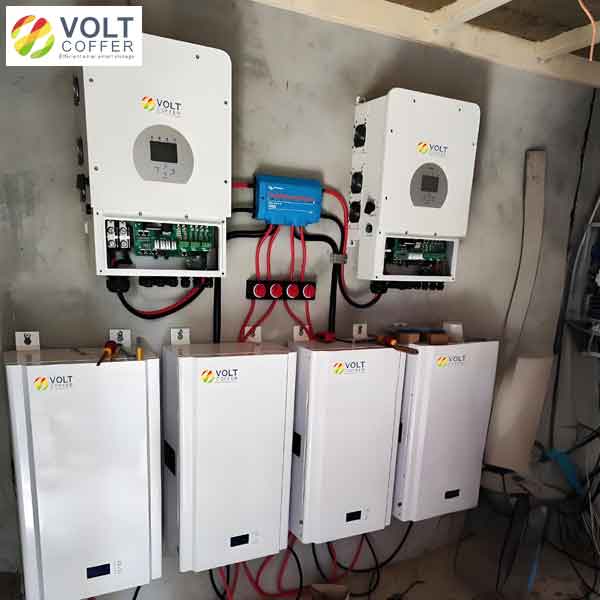
In practical applications, solar inverters like the one shown above often incorporate advanced features such as battery storage integration, highlighting the evolution of cascaded topologies toward hybrid systems. This image exemplifies how modern solar inverters combine multiple technologies to enhance energy management. Returning to the simulation, I further analyzed the output current waveforms, which exhibited smooth sinusoidal shapes due to the inductive load. The current amplitude I_out_fund followed Ohm’s law: $$I_{out\_fund} = \frac{V_{out\_fund}}{\sqrt{R^2 + (2\pi f_m L)^2}}$$ For example, at M=1, with V_out_fund=100 V and load impedance |Z| ≈ 30.1 Ω, I_out_fund ≈ 3.32 A. This calculation aligns with simulation results, verifying the accuracy of the model. The efficiency of solar inverters in such setups can be approximated by considering conduction and switching losses. The total power loss P_loss in the inverter can be expressed as: $$P_{loss} = P_{cond} + P_{sw}$$ where P_cond is conduction loss proportional to current squared, and P_sw is switching loss proportional to switching frequency and voltage. For cascaded solar inverters with CPS-SPWM, P_sw is reduced due to interleaving, as each unit switches at f_c but the effective output frequency is N·f_c. This loss reduction is a significant advantage for high-power solar inverters.
To deepen the analysis, I explored the impact of varying the number of H-bridge units on performance. As N increases, the output voltage levels multiply, following the formula: $$\text{Number of levels} = 2N + 1$$ For N=2, levels = 5; for N=3, levels = 7, and so on. This progression dramatically lowers THD, as shown by the approximate relation: $$\text{THD} \propto \frac{1}{N^2}$$ However, more units require additional DC sources, which in solar inverters could correspond to separate photovoltaic strings or battery banks. This modularity allows solar inverters to be customized for different voltage and power ratings, making them scalable from residential to utility-scale installations. The table below summarizes this scalability for solar inverters.
| Number of Units (N) | Output Voltage Levels | Max Output Voltage (V) | Estimated THD Reduction |
|---|---|---|---|
| 2 | 5 | 2·V_dc | Base |
| 3 | 7 | 3·V_dc | ~44% lower |
| 4 | 9 | 4·V_dc | ~75% lower |
Another critical aspect of solar inverters is their response to non-ideal conditions, such as DC source variations from solar panel shading or temperature changes. In cascaded topologies, if the DC voltages are unequal, the output waveform may become asymmetric, increasing harmonics. To mitigate this, advanced control algorithms like voltage balancing techniques can be incorporated. For instance, a feedback loop can adjust the modulation index for each unit independently, ensuring uniform voltage contribution. This adaptability is a key strength of modern solar inverters, enabling them to maintain high performance despite environmental fluctuations.
In conclusion, my investigation into cascaded multi-level solar inverters demonstrates their superiority in terms of output quality, efficiency, and modularity. Through CPS-SPWM modulation, these solar inverters achieve low harmonic distortion and reduced switching losses, which are essential for grid integration of solar power. The simulation results clearly establish the linear relationship between modulation index and output characteristics, providing a framework for optimizing solar inverters in real-world applications. Future work could focus on implementing more sophisticated control strategies, such as model predictive control or artificial intelligence-based tuning, to further enhance the responsiveness and reliability of solar inverters. As the demand for clean energy grows, advancements in solar inverter technology will continue to play a pivotal role in harnessing solar potential, making systems more efficient and cost-effective.
To summarize the key formulas discussed in this article, I present them in a consolidated manner. These equations are fundamental for designing and analyzing cascaded multi-level solar inverters.
1. Maximum output phase voltage: $$V_{ph\_max} = N \cdot V_{dc}$$
2. Output voltage as superposition: $$v_{out}(t) = \sum_{i=1}^{N} v_i(t)$$
3. Carrier phase shift in CPS-SPWM: $$\Delta \theta = \frac{2\pi}{N}$$
4. Fundamental output voltage amplitude: $$V_{out\_fund} = N \cdot M \cdot V_{dc}$$
5. Output current amplitude: $$I_{out\_fund} = \frac{V_{out\_fund}}{\sqrt{R^2 + (2\pi f_m L)^2}}$$
6. Number of output levels: $$\text{Levels} = 2N + 1$$
7. THD approximation: $$\text{THD} \propto \frac{1}{N^2}$$
These mathematical models, combined with practical simulations, offer a comprehensive understanding of cascaded multi-level solar inverters. By leveraging these insights, engineers can develop more robust and efficient solar inverters, contributing to a sustainable energy future. I hope this detailed exploration encourages further research and innovation in the field of solar inverters, as they are indispensable components in the transition to renewable energy.