
I investigate the coupled electrochemical and mechanical behavior of a solid state cell under externally applied axial pressure, with the goal of identifying a pressure window that balances capacity utilization, interfacial contact recovery, interfacial stress mismatch, and pressurization cost. The solid state cell considered here is a layered thin-film stack in which a positive electrode, a solid polymer electrolyte, and a negative electrode are arranged along the thickness direction. Unlike conventional liquid-electrolyte cells, the solid state cell relies on solid-solid contacts, so the real contact area at the electrode/electrolyte interfaces becomes a first-order variable rather than a fixed geometric quantity. I therefore formulate a pressure-dependent interfacial contact model and couple it to both the interfacial charge-transfer kinetics and the local mechanical load sharing. This coupled path allows the axial pressure to influence the solid state cell through two simultaneous routes: it changes the effective reaction area for interfacial kinetics, and it changes the local elastic bearing stress at the contact spots. The resulting model is used to evaluate a wide pressure range, to construct normalized performance and cost indicators, and to perform multi-criteria optimization under several engineering preferences.
1. Motivation and Scope
Axial pressure is one of the most important operating variables for a solid state cell because it can compress interfacial voids, increase real contact area, reduce interfacial polarization, and improve capacity utilization. However, increasing axial pressure also increases the mechanical load carried by the solid state cell stack, raises the interfacial stress difference between adjacent layers, and imposes higher preload and fixture requirements. The central problem is therefore not whether pressure helps, but how much pressure is beneficial before the electrochemical gains become marginal and the mechanical and engineering costs continue to accumulate. In my analysis, I treat the solid state cell as a one-dimensional layered system under isothermal conditions. This idealization is appropriate for a first-order pressure-window study because the in-plane dimensions are much larger than the thickness, so edge effects and in-plane transport can be neglected under an ideal stacked configuration. The solid state cell is represented by a positive electrode, a solid polymer electrolyte, and a negative electrode, with lithium transport, interfacial charge transfer, chemical strain, and elastic deformation all resolved along the thickness direction.
I focus on four evaluation quantities for the solid state cell: usable areal capacity, minimum interfacial contact factor, maximum interfacial stress difference, and pressurization cost. The first two are benefit-type indicators, while the latter two are cost-type indicators. I normalize each indicator over the pressure range and combine them into a scalar loss function. The pressure that minimizes this loss function is then interpreted as a trade-off optimum for the solid state cell under a given preference. By varying the weights and the mathematical form of the loss function, I test the robustness of the resulting pressure window. I also examine how the pressure window shifts with current density, normalization interval, and interfacial roughness parameters. The final result is a pressure window that is not derived from a single objective but from a systematic multi-criteria compromise for the solid state cell.
2. Coupled Electrochemical–Mechanical Formulation
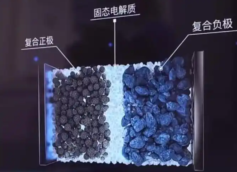
I model the solid state cell as a one-dimensional layered domain along the thickness coordinate \(x\). The positive electrode, solid polymer electrolyte, and negative electrode have natural thicknesses \(l_p\), \(l_e\), and \(l_n\), respectively. The solid state cell is assumed to be isothermal, and the active materials are treated as homogeneous continua. Lithium transport occurs along the thickness direction, and interfacial charge transfer occurs at the two electrode/electrolyte interfaces. The external axial pressure \(P\) is applied along \(x\), and the in-plane directions are assumed to be constrained, so the in-plane strains are zero. The schematic representation of this one-dimensional solid state cell is provided below.
2.1 Lithium transport in electrodes and electrolyte
In the positive and negative electrodes, I describe lithium transport by mass conservation and a stress-coupled flux expression. For \(k=p,n\), the mass balance is
$$ \frac{\partial c_k}{\partial t} + \frac{\partial j_k}{\partial x} = 0, \qquad k=p,n, $$
where \(c_k\) is the lithium concentration and \(j_k\) is the lithium flux. The flux includes both concentration-gradient diffusion and hydrostatic-stress-driven migration:
$$ j_k = -D_k\left(\frac{\partial c_k}{\partial x} – \frac{\Omega_k c_k}{RT}\frac{\partial \sigma_k}{\partial x}\right), \qquad k=p,n. $$
Here \(D_k\) is the lithium diffusion coefficient, \(\Omega_k\) is the partial molar volume, \(\sigma_k\) is the hydrostatic stress, \(R\) is the gas constant, and \(T\) is the temperature. In the solid polymer electrolyte, I use a modified Nernst-Planck description for the lithium concentration \(c_e\) and flux \(j_e\):
$$ \frac{\partial c_e}{\partial t} + \frac{\partial j_e}{\partial x} = 0, $$
$$ j_e = -D_e\left(\frac{\partial c_e}{\partial x} – \frac{\Omega_e c_e}{RT}\frac{\partial \sigma_e}{\partial x}\right) – \frac{i_e}{F}\frac{t_+}{1}. $$
To keep the notation compact, I define the electrolyte diffusion coefficient and partial molar volume as weighted quantities:
$$ D_e = \frac{2D_+D_-}{D_+ + D_-}, $$
$$ \Omega_e = \Omega_+ + \Omega_-. $$
Here \(D_+\) and \(D_-\) are the cation and anion diffusion coefficients, and \(\Omega_+\) and \(\Omega_-\) are the corresponding partial molar volumes. The current density in the electrolyte obeys charge conservation,
$$ \frac{\partial i_e}{\partial x} = 0, $$
and the electrolyte current can be written in a form that contains both concentration and stress contributions. In my numerical implementation, I retain the full one-dimensional transport equations for the solid state cell and solve them together with the mechanical and interfacial equations.
2.2 Interfacial reaction kinetics
At each electrode/electrolyte interface, I describe the charge-transfer reaction by a Butler-Volmer expression. For the positive and negative interfaces,
$$ i_k = i_{k,0}^{\mathrm{eff}} \, 2\sinh\left(\frac{F\eta_k}{2RT}\right), \qquad k=p,n, $$
where \(i_k\) is the interfacial reaction current density, \(\eta_k\) is the interfacial overpotential, and \(i_{k,0}^{\mathrm{eff}}\) is the effective exchange current density. The effective exchange current density includes the pressure-dependent contact factor \(\gamma_{s,k}\):
$$ i_{p,0}^{\mathrm{eff}} = \gamma_{s,p} i_{p,0}, \qquad i_{n,0}^{\mathrm{eff}} = \gamma_{s,n} i_{n,0}. $$
I write the reference exchange current densities as
$$ i_{p,0} = F k_p \left(c_p^{\max} – c_{p,s}\right)^{1-\beta_p} c_{p,s}^{\beta_p} c_{e,s}^{1-\beta_p}, $$
$$ i_{n,0} = F k_n \left(c_n^{\max} – c_{n,s}\right)^{1-\beta_n} c_{n,s}^{\beta_n} c_{e,s}^{1-\beta_n}. $$
Here \(k_p\) and \(k_n\) are reaction rate constants, \(c_{p,s}\) and \(c_{n,s}\) are surface concentrations, \(c_{e,s}\) is the electrolyte lithium concentration at the interface, and \(\beta_p\) and \(\beta_n\) are charge-transfer coefficients. The key coupling in my solid state cell model is that the contact factor \(\gamma_{s,k}\) multiplies the exchange current density. When the real contact area is small, the effective exchange current density is small, so the interfacial overpotential required to sustain a given current density becomes large. This is the electrochemical route by which axial pressure affects the solid state cell.
2.3 Voltage decomposition
To understand which physical process dominates the pressure response, I decompose the terminal voltage of the solid state cell into five contributions:
$$ V_{\mathrm{cell}} = V_{\mathrm{ref}} + V_{\mathrm{con}} + V_{\mathrm{str}} + V_{\mathrm{ove}} + V_{\mathrm{ele}}. $$
The reference voltage is taken as \(V_{\mathrm{ref}} = 3.9\ \mathrm{V}\). The concentration contribution is
$$ V_{\mathrm{con}} = \frac{RT}{F} \ln\left( \frac{c_{e,s} c_{p,s} (c_{n}^{\max}-c_{n,s})}{c_{e,s} c_{n,s} (c_{p}^{\max}-c_{p,s})} \right), $$
and the stress contribution is
$$ V_{\mathrm{str}} = \frac{1}{F}\left( \Omega_p \sigma_{p,s1} – \Omega_n \sigma_{n,s2} + \Omega_e \sigma_{e,s1} – \Omega_e \sigma_{e,s2} \right). $$
The interfacial overpotential contribution is
$$ V_{\mathrm{ove}} = \eta_p – \eta_n, $$
and the electrolyte potential contribution is
$$ V_{\mathrm{ele}} = \phi_{e,s1} – \phi_{e,s2}. $$
In my simulations, \(V_{\mathrm{ele}}\) is very small, so the main pressure-sensitive terms are \(V_{\mathrm{ove}}\), \(V_{\mathrm{str}}\), and \(V_{\mathrm{con}}\). The decomposition is useful because it shows whether pressure improves the solid state cell primarily by reducing interfacial polarization or by changing bulk transport and thermodynamic contributions.
| Component | Physical meaning | Main sensitivity |
|---|---|---|
| \(V_{\mathrm{ref}}\) | Reference potential | Material system |
| \(V_{\mathrm{con}}\) | Concentration polarization | State of charge |
| \(V_{\mathrm{str}}\) | Stress contribution | Chemical strain and pressure |
| \(V_{\mathrm{ove}}\) | Interfacial overpotential | Contact factor and current density |
| \(V_{\mathrm{ele}}\) | Electrolyte potential drop | Ion transport |
2.4 Mechanical equilibrium and chemical strain
The mechanical response of the solid state cell is obtained from the equilibrium equation
$$ \nabla \cdot \sigma + b = 0. $$
I apply an axial pressure \(P\) along \(x\), so the thickness-direction stress is \(\sigma_{xx} = -P\). I further assume that the in-plane strains are zero, \(\varepsilon_{yy}=\varepsilon_{zz}=0\). The total strain in each layer is decomposed into an elastic part and a chemical part:
$$ \varepsilon = \varepsilon^{\mathrm{elas}} + \varepsilon^{\mathrm{chem}}. $$
For layer \(k=p,n,e\), the chemical strain is related to the concentration change by
$$ \varepsilon_k^{\mathrm{chem}} = \frac{\Omega_k}{3}\left(c_k – c_k^0\right). $$
Using linear isotropic elasticity under the plane-strain-like constraint, the hydrostatic stress in layer \(k\) can be written as
$$ \sigma_k = -\frac{P E_k}{3(1-\nu_k)} + \frac{E_k \Omega_k}{9(1-\nu_k)}\left(c_k – c_k^0\right), $$
where \(E_k\) is Young’s modulus and \(\nu_k\) is Poisson’s ratio. The exact coefficient depends on the assumed constraint condition, but the structure of the expression is what matters for the solid state cell: the first term is the external-pressure contribution, and the second term is the chemical-expansion contribution. The layer strain is then
$$ \varepsilon_k = \frac{(1+\nu_k)(1-2\nu_k)}{E_k}P + \frac{\Omega_k}{3}\left(c_k – c_k^0\right). $$
The total thickness change of the solid state cell is
$$ \Delta l = \varepsilon_p l_p + \varepsilon_e l_e + \varepsilon_n l_n. $$
I also evaluate the maximum thickness variation during operation, defined as
$$ H(P) = \max_t l(P,t) – \min_t l(P,t). $$
This quantity is useful for interpreting the breathing response of the solid state cell, although its absolute magnitude is small relative to the total thickness.
2.5 Pressure-dependent interfacial contact
The solid state cell interfaces are not perfectly conformal. Because the electrode and electrolyte surfaces are rough and have different elastic properties, the real contact area \(A\) is smaller than the nominal area \(A_0\). I define the interfacial contact factor as
$$ \gamma = \frac{A}{A_0}. $$
I use a Persson-type contact description to relate \(\gamma\) to the nominal contact pressure. In general form,
$$ \gamma = \int_{q_L}^{q_0} \mathrm{erf}\left(\frac{q E^*}{\sqrt{2}\sigma_0}\right) C(q) \, dq, $$
where \(E^*\) is the effective modulus, \(\sigma_0\) is the nominal contact stress, \(C(q)\) is the power spectral density of the rough surface, and \(q_L\) and \(q_0\) are the lower and upper cutoff wavenumbers. The effective modulus is
$$ \frac{1}{E^*} = \frac{1-\nu_1^2}{E_1} + \frac{1-\nu_2^2}{E_2}. $$
I take the roughness spectrum in the form
$$ C(q) = 10^{m} q^{I}, $$
where \(m\) and \(I\) are roughness parameters. For the positive electrode/electrolyte interface, I use film-type parameters, and for the negative electrode/electrolyte interface, I use bulk-type parameters. The contact factor is then coupled back into the electrochemical model through the effective exchange current density, and it is also coupled into the mechanical model through the local bearing stress. Specifically, the elastic part of the interfacial stress is amplified by \(1/\gamma_{s,k}\):
$$ \sigma_{k,sj}^{\mathrm{eff}} = \frac{1}{\gamma_{s,k}} \sigma_{k,sj}^{\mathrm{elas}} + \sigma_{k,sj}^{\mathrm{chem}}, \qquad j=1,2. $$
The interfacial stress difference is defined as
$$ \Delta \sigma_{s1}^{\mathrm{eff}} = \left| \sigma_{p,s1}^{\mathrm{eff}} – \sigma_{e,s1}^{\mathrm{eff}} \right|, $$
$$ \Delta \sigma_{s2}^{\mathrm{eff}} = \left| \sigma_{n,s2}^{\mathrm{eff}} – \sigma_{e,s2}^{\mathrm{eff}} \right|. $$
These quantities measure the mechanical mismatch across the solid state cell interfaces. A large interfacial stress difference indicates that the two sides of the interface respond differently to the same electrochemical and mechanical loading, which is a potential reliability concern for the solid state cell.
2.6 Parameter set
The main material and operating parameters used in my solid state cell model are listed below.
| Parameter | Positive electrode | Solid polymer electrolyte | Negative electrode |
|---|---|---|---|
| Thickness (nm) | 550 | 2000 | 200 |
| Maximum concentration (mol/m³) | 23300 | 1500 | 30555 |
| Initial concentration (mol/m³) | 22135 | 1200 | 1527.75 |
| Reaction rate constant (m²·⁵ mol⁻⁰·⁵ s⁻¹) | 1.53×10⁻¹¹ | — | 5.03×10⁻¹¹ |
| Diffusion coefficient (m²/s) | 1.76×10⁻¹⁵ | 2.5×10⁻¹³ (cation), 3×10⁻¹³ (anion) | 8×10⁻¹⁴ |
| Partial molar volume (m³/mol) | 1.92×10⁻⁶ | 3.95×10⁻⁶ (cation), 1.46×10⁻⁴ (anion) | 4.17×10⁻⁶ |
| Charge-transfer coefficient | 0.5 | — | 0.5 |
| Young’s modulus (GPa) | 70 | 0.5 | 10 |
| Poisson’s ratio | 0.20 | 0.40 | 0.30 |
I set the temperature to \(T=300\ \mathrm{K}\) and the reference concentration to \(c_{\mathrm{ref}}=1\ \mathrm{mol/m^3}\). The solid state cell is charged at \(1\ \mathrm{A/m^2}\) to a cutoff voltage of \(4.03\ \mathrm{V}\), and then discharged at the same current density until the state of charge reaches 0.05. The pressure scan uses a spacing of 0.3 MPa below 4 MPa and 1 MPa above 4 MPa.
3. Numerical Implementation and Verification
I solve the coupled equations in COMSOL Multiphysics using a fully coupled solver and the MUMPS linear solver. The relative tolerance is 0.005, and the tolerance factor is 0.1. To ensure that the results are not artifacts of discretization or time stepping, I perform mesh-independence, time-step-independence, and roughness-parameter sensitivity studies. I also compare my model structure with several existing modeling approaches for solid state cell systems.
3.1 Comparison with existing model structures
| Model type | Main additional feature |
|---|---|
| Stress-coupled transport model | Couples hydrostatic stress into transport and interfacial kinetics and studies bending loads |
| Contact-loss model | Introduces Persson contact theory and a contact factor into interfacial kinetics |
| Composite-electrode model | Includes pressure effects on microstructure, porosity, and effective transport parameters |
| My present model | Couples axial pressure through the contact factor into exchange current density, hydrostatic stress, and interfacial stress difference |
The main novelty of my formulation is that it treats the axial pressure as a variable that simultaneously changes the interfacial reaction area and the local elastic bearing stress. In this way, the solid state cell response is not merely a superposition of an electrochemical model and a mechanical model; the contact state is an internal variable that links the two.
3.2 Validation of the baseline electrochemical behavior
To validate the baseline behavior, I set both contact factors to unity and compare the terminal voltage versus state of charge with a reference solid state cell model using the same material system. The agreement is quantified by a coefficient of determination of \(R^2 = 0.9931\) and a maximum absolute voltage error of \(0.0310\ \mathrm{V}\). The voltage plateau, the state-of-charge range, and the high-state-of-charge voltage variation are all reproduced. This supports the use of my model for the subsequent pressure analysis of the solid state cell.
I also compare the pressure sensitivity of the charge-transfer resistance. The area coefficient in the contact model is defined as
$$ n = \frac{d\ln R_{\mathrm{int}}}{d\ln \gamma}. $$
In my formulation, the interfacial resistance scales as
$$ R_{\mathrm{int}} = \frac{RT}{F i_0^{\mathrm{eff}}} = \frac{RT}{F \gamma i_0}. $$
Therefore, the area coefficient is \(-1\). Experimental reports for ceramic solid electrolytes give values in the range \(-1.13\) to \(-1.05\), which is close to my model response. I further define a normalized charge-transfer resistance
$$ R_{\mathrm{norm}}(P) = \frac{R_{\mathrm{ct}}(P)}{R_{\mathrm{ct}}(P_0)}, $$
where \(R_{\mathrm{ct}}\) is the total charge-transfer resistance of the solid state cell. For a pressure change from a low reference pressure to about 1.2 MPa, my model gives \(R_{\mathrm{norm}} = 0.7041\), while an experimental reference gives \(0.7326\). The difference is small, which supports the pressure sensitivity of my interfacial contact coupling.
3.3 Mesh and time-step independence
I use five mesh levels for the solid state cell. The numbers of elements in the positive electrode, electrolyte, and negative electrode are listed below.
| Scheme | Positive electrode | Electrolyte | Negative electrode | Total |
|---|---|---|---|---|
| M1 | 14 | 18 | 10 | 42 |
| M2 | 21 | 27 | 15 | 63 |
| M3 | 35 | 45 | 25 | 105 |
| M4 | 70 | 90 | 50 | 210 |
| M5 | 140 | 180 | 100 | 420 |
Across these mesh schemes, the maximum voltage deviation is only \(0.274\ \mathrm{mV}\), and the maximum deviation in the positive-electrode/electrolyte interfacial stress difference at 10 MPa is \(0.111\ \mathrm{MPa}\). These deviations are small relative to the corresponding signal magnitudes, so I adopt the M1 scheme with uniform elements in each layer.
I also examine five maximum time steps: 2 s, 1 s, 0.5 s, 0.25 s, and 0.125 s. The maximum voltage deviation is \(0.53\ \mathrm{mV}\), and the interfacial stress difference is almost unchanged. For the solid state cell simulations, I therefore use a maximum time step of 2 s to balance accuracy and computational cost.
| Scheme | Maximum time step |
|---|---|
| T1 | 2 s |
| T2 | 1 s |
| T3 | 0.5 s |
| T4 | 0.25 s |
| T5 | 0.125 s |
3.4 Roughness-parameter sensitivity
I vary the roughness parameters \(m\) and \(I\) over a wider range to examine whether the pressure-window conclusions depend on a particular surface description. The schemes are listed below.
| Scheme | Positive interface \(m\) / negative interface \(m\) | Positive interface \(I\) / negative interface \(I\) |
|---|---|---|
| R1 | -2.77 / -3.08 | -9.35 / -6.61 |
| R2 | -2.67 / -2.98 | -10.35 / -7.61 |
| R3 | -2.72 / -3.03 | -9.85 / -7.11 |
| R4 | -2.82 / -3.13 | -8.85 / -6.11 |
| R5 | -2.87 / -3.18 | -8.35 / -5.61 |
As the roughness increases, the contact factor recovers more slowly with pressure. At low pressure, the charge-discharge curves differ noticeably among the roughness schemes, but at medium and high pressure the differences become small. The maximum interfacial stress difference also decreases as roughness increases, but its monotonic increasing trend with pressure remains. Therefore, the roughness parameters affect the low-pressure response and the numerical values of the indicators, but they do not change the main qualitative conclusion: the solid state cell requires a moderate pressure window to balance contact recovery and mechanical cost.
4. Electrochemical and Mechanical Response to Axial Pressure
In this section I analyze how the solid state cell responds to axial pressure. I separate the discussion into interfacial contact, terminal voltage and capacity, voltage components, layer stress, interfacial stress difference, and thickness variation. The purpose is to identify which quantities are most sensitive to pressure and which quantities become limiting at high pressure.
4.1 Interfacial contact factor
Both the positive-electrode/electrolyte interface and the negative-electrode/electrolyte interface show a fast increase in contact factor at low pressure, followed by saturation at higher pressure. However, the two interfaces do not respond identically. The positive interface approaches nearly full contact at a relatively low pressure, while the negative interface requires a higher pressure to reach a similar level. This means that the minimum contact factor among the two interfaces,
$$ \gamma_{\min}(P) = \min\left(\gamma_{s1}(P), \gamma_{s2}(P)\right), $$
is controlled by the negative side over much of the pressure range. This minimum contact factor is a natural benefit indicator for the solid state cell because it represents the weaker interface.
4.2 Terminal voltage and capacity
For a given state of charge, increasing the contact factor shifts the discharge curve to higher voltage and higher capacity. In a constant-current discharge, a small contact factor means that the same current must be carried by a smaller effective reaction area. The local interfacial current density therefore increases, the overpotential increases, and the terminal voltage reaches the cutoff condition earlier. As a result, the usable areal capacity of the solid state cell decreases. When the contact factor is large, the effective reaction area increases, the interfacial overpotential decreases, and the solid state cell can sustain a higher terminal voltage for a longer portion of the discharge. The usable areal capacity is therefore larger.
I define the areal capacity as
$$ Q(P) = \frac{i_{\mathrm{app}} t_{\mathrm{cut}}(P)}{3600}, $$
where \(i_{\mathrm{app}}\) is the applied current density and \(t_{\mathrm{cut}}\) is the discharge time. The pressure dependence of \(Q\) is strong at low pressure and becomes weak at high pressure. This is the first indication of diminishing electrochemical returns for the solid state cell.
4.3 Voltage-component contributions
The voltage decomposition reveals that the concentration contribution is mainly controlled by the state of charge and is only weakly affected by pressure. The stress contribution increases with the state of charge and slightly increases with pressure, but its magnitude is only tens of millivolts. The interfacial overpotential contribution is the most pressure-sensitive term. At low pressure, the poor contact state forces the solid state cell to operate with a large interfacial overpotential, so the overpotential contribution is large. As pressure increases, the contact factor increases, the effective exchange current density increases, and the overpotential contribution decreases. This is the main route by which axial pressure improves the terminal voltage and capacity utilization of the solid state cell.
I define the absolute share of a voltage component as
$$ \chi_i = \frac{|V_i|}{|V_{\mathrm{con}}| + |V_{\mathrm{str}}| + |V_{\mathrm{ove}}|} \times 100\%, \qquad i=\mathrm{con},\mathrm{str},\mathrm{ove}. $$
At two representative states of charge, the share of the overpotential contribution decreases strongly with pressure, while the share of the concentration contribution increases. The latter increase is mainly a relative effect: once the overpotential contribution is reduced, the concentration contribution occupies a larger fraction of the remaining voltage loss. The stress contribution remains a minor correction term. Therefore, the solid state cell benefits from pressure mainly because interfacial polarization is reduced, not because the bulk concentration or stress contributions are fundamentally changed.
| Component | Pressure sensitivity | Role |
|---|---|---|
| Concentration contribution | Weak | Mainly follows state of charge |
| Stress contribution | Moderate but small in magnitude | Correction term |
| Overpotential contribution | Strong | Dominant pressure-sensitive loss |
| Electrolyte potential contribution | Very weak | Negligible in this solid state cell |
4.4 Layer stress and interfacial stress difference
The layer stress distribution depends strongly on the state of charge. As the state of charge increases, the positive electrode becomes more tensile, and the negative electrode becomes more compressive, while the electrolyte stress remains relatively small. This behavior is caused by the different chemical strains and elastic properties of the three layers. At the same state of charge, the direct effect of axial pressure on the layer stress distribution is relatively limited: increasing pressure from 0.1 MPa to 1 MPa causes only small changes, while increasing pressure to 10 MPa or 50 MPa slightly increases the compressive stress in the electrolyte and negative electrode. The positive electrode tensile stress is almost unchanged. This shows that the internal stress state of the solid state cell is not controlled by external pressure alone; it is a combined result of pressure, concentration, and material mismatch.
The interfacial stress difference, however, increases monotonically with pressure. At low pressure, the interfacial stress difference rises quickly, and then the growth slows down. This behavior has two causes. First, under incomplete contact, the nominal pressure is carried mainly by the real contact spots, so the local bearing stress is amplified. As pressure increases, the contact factor increases, and the local amplification is reduced. Second, higher pressure allows the solid state cell to operate over a wider state-of-charge range, so the chemical strain at high state of charge becomes larger. The positive-electrode/electrolyte interface has a higher maximum interfacial stress difference than the negative-electrode/electrolyte interface, and it continues to increase more noticeably at high pressure. Therefore, the positive interface is the more mechanically critical interface in my solid state cell model. This is why I use the maximum interfacial stress difference as a cost indicator in the pressure optimization.
4.5 Thickness variation
The maximum thickness variation \(H\) is defined as
$$ H(P) = \max_t l(P,t) – \min_t l(P,t). $$
As pressure increases, \(H\) first increases and then levels off. The increase is noticeable from 0.1 MPa to about 4 MPa, where \(H\) rises from roughly 4 nm to 8 nm. At higher pressure, the curve becomes flat, and the differences between pressure levels become small. The reason is that low pressure limits the accessible state-of-charge range, so the concentration change and chemical strain are small. As pressure improves contact and reduces polarization, the solid state cell can access a wider state-of-charge range, so the thickness breathing increases. Once contact and capacity improvements saturate, the thickness variation also saturates. Although \(H\) is sensitive to pressure at low pressure, its absolute magnitude is only a few nanometers, which is small relative to the total thickness of the solid state cell. Therefore, I treat \(H\) as a supplementary mechanical response rather than a primary optimization objective.
5. Multi-Criteria Pressure Window Optimization
The pressure window of the solid state cell cannot be determined from a single metric. A high pressure may improve capacity and contact, but it also increases interfacial stress difference and pressurization cost. I therefore construct a multi-criteria loss function and search for the pressure that minimizes it. I use four normalized indicators: usable areal capacity, minimum interfacial contact factor, maximum interfacial stress difference, and axial pressure itself as a proxy for pressurization cost.
5.1 Normalized indicators and loss function
The normalized capacity indicator is
$$ Q_n(P) = \frac{Q(P)-Q_{\min}}{Q_{\max}-Q_{\min}}. $$
The normalized minimum contact factor is
$$ \gamma_{n,\min}(P) = \frac{\gamma_{\min}(P)-\gamma_{\min}^{\min}}{\gamma_{\min}^{\max}-\gamma_{\min}^{\min}}. $$
The normalized maximum interfacial stress difference is
$$ S_n(P) = \frac{S(P)-S_{\min}}{S_{\max}-S_{\min}}, $$
where
$$ S(P) = \max\left( \left|\sigma_{p,s1}^{\mathrm{eff}}-\sigma_{e,s1}^{\mathrm{eff}}\right|, \left|\sigma_{n,s2}^{\mathrm{eff}}-\sigma_{e,s2}^{\mathrm{eff}}\right| \right). $$
The normalized pressure cost is
$$ P_n(P) = \frac{P-P_{\min}}{P_{\max}-P_{\min}}, $$
with \(P_{\min}=0.1\ \mathrm{MPa}\) and \(P_{\max}=50\ \mathrm{MPa}\). The total loss function is
$$ J(P) = J_Q + J_\gamma + J_S + J_P, $$
where the components are
$$ J_Q = w_Q \left[1-Q_n(P)\right]^2, $$
$$ J_\gamma = w_\gamma \left[1-\gamma_{n,\min}(P)\right]^2, $$
$$ J_S = w_S S_n(P), $$
$$ J_P = w_P P_n(P). $$
The weights \(w_Q\), \(w_\gamma\), \(w_S\), and \(w_P\) represent the relative importance of capacity, contact recovery, interfacial stress difference, and pressurization cost. I consider three preference schemes: performance priority, balanced, and conservative. The weights are listed below.
| Scheme | \(w_Q\) | \(w_\gamma\) | \(w_S\) | \(w_P\) |
|---|---|---|---|---|
| Performance priority | 0.35 | 0.40 | 0.15 | 0.10 |
| Balanced | 0.30 | 0.35 | 0.20 | 0.15 |
| Conservative | 0.25 | 0.30 | 0.25 | 0.20 |
5.2 Particle swarm and deterministic search
Because the loss function depends on the full numerical solution of the solid state cell model, I do not use an analytical gradient. I perform a derivative-free bounded search using particle swarm optimization. Each particle position is a candidate axial pressure. The velocity and position updates are
$$ v_i^{k+1} = \omega v_i^k + c_1 r_1 \left(p_i^k – P_i^k\right) + c_2 r_2 \left(g^k – P_i^k\right), $$
$$ P_i^{k+1} = P_i^k + v_i^{k+1}. $$
I use 15 particles and 9 iterations. The inertia weight is 0.65, and the individual and group learning factors are both 1.45. The velocity limit is 8 MPa. For each candidate pressure, the solid state cell model is solved again, and the normalized indicators are recomputed. I then refine the result by a local scan around the best pressure.
To verify that the result is not algorithm-specific, I also use a deterministic method combining a coarse full-range scan with one-dimensional bounded optimization. The coarse scan uses 1 MPa intervals from 0.1 MPa to 50 MPa. A node is selected as a local minimum candidate if
$$ J(P_i) \leq \min\left(J(P_{i-1}),J(P_{i+1})\right). $$
Each candidate interval is then refined by a bounded one-dimensional optimizer. The final optimum is
$$ P^* = \arg\min_{P\in\{P_{\min},P_{\max},P_1^*,\dots,P_m^*\}} J(P). $$
The pressure convergence tolerance is \(10^{-3}\ \mathrm{MPa}\), and the maximum number of function evaluations is 500.
5.3 Optimization results
The two search methods give very similar optimal pressures. The particle swarm results are listed below.
| Preference | Trade-off optimal pressure |
|---|---|
| Performance priority | 15.8 MPa |
| Balanced | 12.2 MPa |
| Conservative | 10.0 MPa |
The deterministic coarse-scan and bounded-optimization results are listed below.
| Preference | Trade-off optimal pressure |
|---|---|
| Performance priority | 15.7 MPa |
| Balanced | 12.4 MPa |
| Conservative | 9.8 MPa |
The difference between the two methods is at most 0.2 MPa in all three schemes. This confirms that the pressure-window result is not an artifact of a particular optimizer. Because the model has no analytical gradient and may later be extended to multiple design variables, I use the particle swarm results for the subsequent discussion. The corresponding key indicators are listed below.
| Scheme | \(Q\) (Ah/m²) | \(\gamma_{\min}\) | \(S\) (MPa) | \(P\) (MPa) |
|---|---|---|---|---|
| Performance priority | 0.1368 | 0.8079 | 579.25 | 15.8 |
| Balanced | 0.1342 | 0.7471 | 574.93 | 12.2 |
| Conservative | 0.1316 | 0.6971 | 569.51 | 10.0 |
In the balanced scheme, the capacity term and contact term dominate the loss at low pressure. As pressure increases, both terms decrease rapidly. At higher pressure, the capacity term is already close to its minimum, and the contact term decreases more slowly, while the interfacial stress difference term and the pressure cost term continue to increase. As a result, the total loss reaches a minimum near 12.2 MPa. This pressure represents a compromise among capacity, contact recovery, interfacial stress difference, and pressurization cost for the solid state cell.
5.4 Marginal benefit and marginal cost
To further interpret the pressure window, I define a normalized benefit indicator as
$$ B(P) = \frac{Q_n(P) + \gamma_{n,\min}(P)}{2}, $$
and a normalized cost indicator as
$$ C(P) = \frac{S_n(P) + P_n(P)}{2}. $$
I then compute the changes \(\Delta B\) and \(\Delta C\) for an additional 1 MPa of axial pressure. At low pressure, the marginal benefit of increasing pressure is high. As pressure increases, the marginal benefit decreases quickly and becomes almost zero in the medium-pressure range. In contrast, the marginal cost remains positive over a wide pressure range because the interfacial stress difference and the pressurization cost continue to accumulate. Near 12 MPa, the marginal benefit and marginal cost are close to each other. Beyond that point, the additional electrochemical benefit is limited, while the cost continues to grow. This confirms the dual role of axial pressure in the solid state cell.
Taken together, the normalized indicator curves, the marginal benefit and cost curves, and the multi-scheme optimization results suggest a trade-off pressure window of 10.0–15.8 MPa for the solid state cell under the present material system and ideal layered structure. The balanced trade-off optimum is 12.2 MPa. Within this window, the solid state cell can maintain good capacity output and interfacial contact while avoiding excessive accumulation of interfacial stress difference and pressure cost.
6. Sensitivity and Robustness
I test whether the pressure window is robust to changes in weighting, normalization interval, loss-function form, and current density. This is important because the solid state cell pressure window should not depend on a single arbitrary modeling choice.
6.1 Weight perturbation
I generate 5000 random weight combinations satisfying
$$ 0.18 \leq w_Q \leq 0.45, $$
$$ 0.20 \leq w_\gamma \leq 0.50, $$
$$ 0.08 \leq w_S \leq 0.35, $$
$$ 0.05 \leq w_P \leq 0.30, $$
with the four weights summing to one. The random sampling uses a Dirichlet distribution with parameter vector \((3,3,2,2)\), followed by rejection filtering according to the above bounds. The resulting distribution of optimal pressure has 5%, 25%, 50%, 75%, and 95% quantiles of 7.12 MPa, 9.10 MPa, 11.10 MPa, 13.81 MPa, and 17.92 MPa, respectively. The median optimal pressure is 11.10 MPa, which is close to the balanced optimum of 12.2 MPa. About 63.56% of the samples fall within the trade-off pressure window of 10.0–15.8 MPa. This indicates that the moderate-pressure window is not an accidental result of one particular weight set for the solid state cell.
6.2 Normalization interval
I also test three normalization intervals: the original interval \([0.1,50]\ \mathrm{MPa}\), an upper-expanded interval \([0.1,60]\ \mathrm{MPa}\), and a 5%–95% quantile interval \([2.6,47.5]\ \mathrm{MPa}\). The results are listed below.
| Normalization interval | Trade-off pressure window |
|---|---|
| Original | 10.0–15.8 MPa |
| Upper expanded by 20% | 10.8–17.1 MPa |
| 5%–95% quantile | 11.8–17.9 MPa |
The window shifts somewhat, but it remains in the medium-pressure range and overlaps substantially with the original window. Therefore, the solid state cell pressure window is reasonably robust to the normalization interval.
6.3 Loss-function form
I test a fully quadratic loss, a normalized Huber loss with threshold \(\delta=0.5\), and an exponential loss. The Huber function is
$$ H(x) = \begin{cases} \frac{2}{3}x^2, & 0 \leq x \leq 0.5, \\ \frac{4}{3}x – \frac{1}{3}, & 0.5 < x \leq 1, \end{cases} $$
and the exponential function is
$$ E(x) = \frac{1-e^{-2x}}{1-e^{-2}}. $$
The corresponding loss forms are
$$ J_{\mathrm{Huber}}(P) = w_Q H(1-Q_n(P)) + w_\gamma H(1-\gamma_{n,\min}(P)) + w_S H(S_n(P)) + w_P H(P_n(P)), $$
$$ J_{\mathrm{exp}}(P) = w_Q E(1-Q_n(P)) + w_\gamma E(1-\gamma_{n,\min}(P)) + w_S E(S_n(P)) + w_P E(P_n(P)). $$
The optimization results are listed below.
| Loss-function form | Trade-off pressure window |
|---|---|
| Original form | 10.0–15.8 MPa |
| Fully quadratic | 11.5–16.7 MPa |
| Normalized Huber | 12.8–17.5 MPa |
| Exponential | 11.0–18.6 MPa |
Although the endpoints change, all windows lie in the medium-pressure range and overlap with the original window. The solid state cell pressure window is therefore not highly sensitive to the mathematical form of the loss function.
6.4 Current density
I also optimize the pressure window at different charge-discharge current densities. The results are listed below.
| Current density | Trade-off pressure window |
|---|---|
| 1 A/m² | 10.0–15.8 MPa |
| 0.135 A/m² | 8.8–14.0 MPa |
| 0.270 A/m² | 9.3–14.9 MPa |
| 0.406 A/m² | 9.6–15.4 MPa |
| 0.541 A/m² | 9.8–15.6 MPa |
| 0.744 A/m² | 9.9–15.8 MPa |
Lower current densities shift the pressure window slightly toward lower pressure, but the change is small. The window remains in the medium-pressure range. This further supports the robustness of the pressure window for the solid state cell.
6.5 Engineering preload implication
For a large-format solid state cell, the axial pressure must be translated into a preload force. If the cell area is \(A\), the preload force is
$$ F = P A. $$
Using a representative large-format pouch area of \(120\ \mathrm{mm} \times 80\ \mathrm{mm}\), the trade-off pressure window of 10.0–15.8 MPa corresponds to a total preload force of about 96.0–151.7 kN. The balanced pressure of 12.2 MPa corresponds to about 117.1 kN. This is a substantial preload requirement, and it places demands on end plates, fasteners, and fixture stiffness. The pressure window also lies within the clamping pressure range reported for high-pressure solid state cell fixtures. If the end-plate and clamping design are appropriate, the pressure uniformity can remain acceptable. However, the present model does not include module-level structural stress, yield safety factors, or pressure nonuniformity. Therefore, the pressure window should be understood as a trade-off result for the present material parameters, ideal layered structure, and evaluation preferences. Application to a practical solid state cell or module requires further design and verification.
7. Conclusions
I have developed a coupled electrochemical-mechanical model for a solid state cell that includes axial pressure, pressure-dependent interfacial contact, and interfacial stress mismatch. The model couples the contact factor into both the interfacial exchange current density and the local elastic bearing stress. Using this model, I evaluated the electrochemical and mechanical response of the solid state cell over a wide pressure range and performed multi-criteria pressure-window optimization. The main conclusions are as follows.
First, axial pressure improves the electrochemical performance of the solid state cell mainly by increasing the real interfacial contact area and reducing interfacial polarization. At low pressure, the effective reaction area is limited, the interfacial charge-transfer overpotential is large, and the terminal voltage and usable capacity are reduced. As pressure increases, the contact factor increases, the overpotential contribution decreases, and the voltage and capacity improve. However, the electrochemical benefit shows diminishing returns. Once the contact factor approaches saturation, further pressure increases produce only small gains in voltage and capacity. Therefore, a moderate pressure is necessary for maintaining solid-solid contact in the solid state cell, but excessive pressure does not continue to improve the electrochemical output significantly.
Second, axial pressure affects the mechanical response by changing layer stress, increasing the interfacial stress difference, and altering thickness variation. The layer stress distribution is mainly controlled by the state of charge and chemical strain, while the direct effect of pressure at a fixed state of charge is limited. The maximum interfacial stress difference increases monotonically with pressure, and the positive-electrode/electrolyte interface shows a higher stress difference than the negative-electrode/electrolyte interface. The maximum thickness variation increases at low pressure but tends to level off at high pressure. Its absolute magnitude is small, so it is not the main limiting factor. The interfacial stress difference is a more meaningful mechanical cost indicator for high-pressure operation of the solid state cell.
Third, the multi-criteria optimization based on usable areal capacity, minimum interfacial contact factor, maximum interfacial stress difference, and pressurization cost yields a trade-off pressure window of 10.0–15.8 MPa for the present material system, ideal layered structure, and isothermal conditions. The balanced trade-off optimum is 12.2 MPa. This window provides a reasonable balance between electrochemical performance and mechanical/engineering cost. It is robust to weight perturbation, normalization interval, loss-function form, and current density within the ranges examined. The results provide a modeling and evaluation framework for pressure regulation and interfacial reliability analysis of multilayer-integrated solid state cell systems. Future work should incorporate real rough interfaces, interfacial damage evolution, debonding, local contact failure, temperature effects, extreme operating conditions, and module-level structural constraints such as end-plate stiffness, mass, and pressure uniformity.
| Quantity | Low-pressure behavior | Medium-pressure behavior | High-pressure behavior |
|---|---|---|---|
| Capacity | Limited by poor contact | Rapidly improving | Saturated |
| Contact factor | Low | Increasing | Near saturation |
| Overpotential | Large | Decreasing | Small and stable |
| Interfacial stress difference | Rising quickly | Rising moderately | Still increasing |
| Thickness variation | Small | Increasing | Nearly flat |
| Pressure cost | Low | Moderate | High |
Overall, my analysis shows that the solid state cell pressure window should be selected by balancing electrochemical benefit against mechanical and engineering cost. The trade-off pressure window identified here is not a universal constant; it depends on the material system, interfacial roughness, mechanical properties, and operating conditions. Nevertheless, the coupled modeling and multi-criteria optimization approach provides a systematic way to determine a defensible pressure window for a solid state cell and to compare different pressure-management strategies.