
The global imperative to mitigate climate change has catalyzed a widespread commitment to carbon neutrality, with numerous nations, including China, establishing ambitious targets for peak carbon emissions and ultimate carbon neutrality. A pivotal strategy in this transition is the restructuring of the energy mix to significantly elevate the proportion of electricity generated from non-fossil fuel sources. Electrochemical energy storage systems (ESS) have emerged as a critical enabling technology for integrating intermittent renewable energy. Among available technologies, lithium-ion batteries dominate the installed capacity landscape. Within this domain, the lithium iron phosphate (LiFePO4) battery, prized for its safety, long cycle life, and declining cost, has become the predominant choice for large-scale stationary storage applications, constituting over 94% of deployments in grid-side, generation-side, and user-side scenarios.
As LiFePO4 battery systems scale to megawatt-hour levels, ensuring their operational performance, longevity, and, most critically, safety becomes paramount. A fundamental challenge arises from the inherent inconsistencies among individual cells within a battery pack. These inconsistencies, stemming from minor variations in manufacturing, operating temperatures, and aging, manifest as divergences in capacity, internal resistance, and state-of-charge (SOC) during operation. The “bucket effect” or “short-board effect” is a direct consequence: the cell with the smallest capacity or highest impedance in a series string limits the usable capacity of the entire string. This weakest cell charges and discharges faster than its peers, leading to accelerated aging and posing potential safety risks if driven beyond its safe operating window. While passive or active balancing circuits can mitigate SOC imbalances, they cannot restore lost capacity or repair a fundamentally degraded “short-board” cell, which ultimately requires replacement. Therefore, a pressing need exists for an engineered, online, rapid, and accurate methodology to detect, classify, and locate inconsistent cells—particularly those evolving into short-board cells—within an operational ESS. Such a capability is indispensable for proactive system maintenance, optimizing usable capacity, and preempting safety hazards.
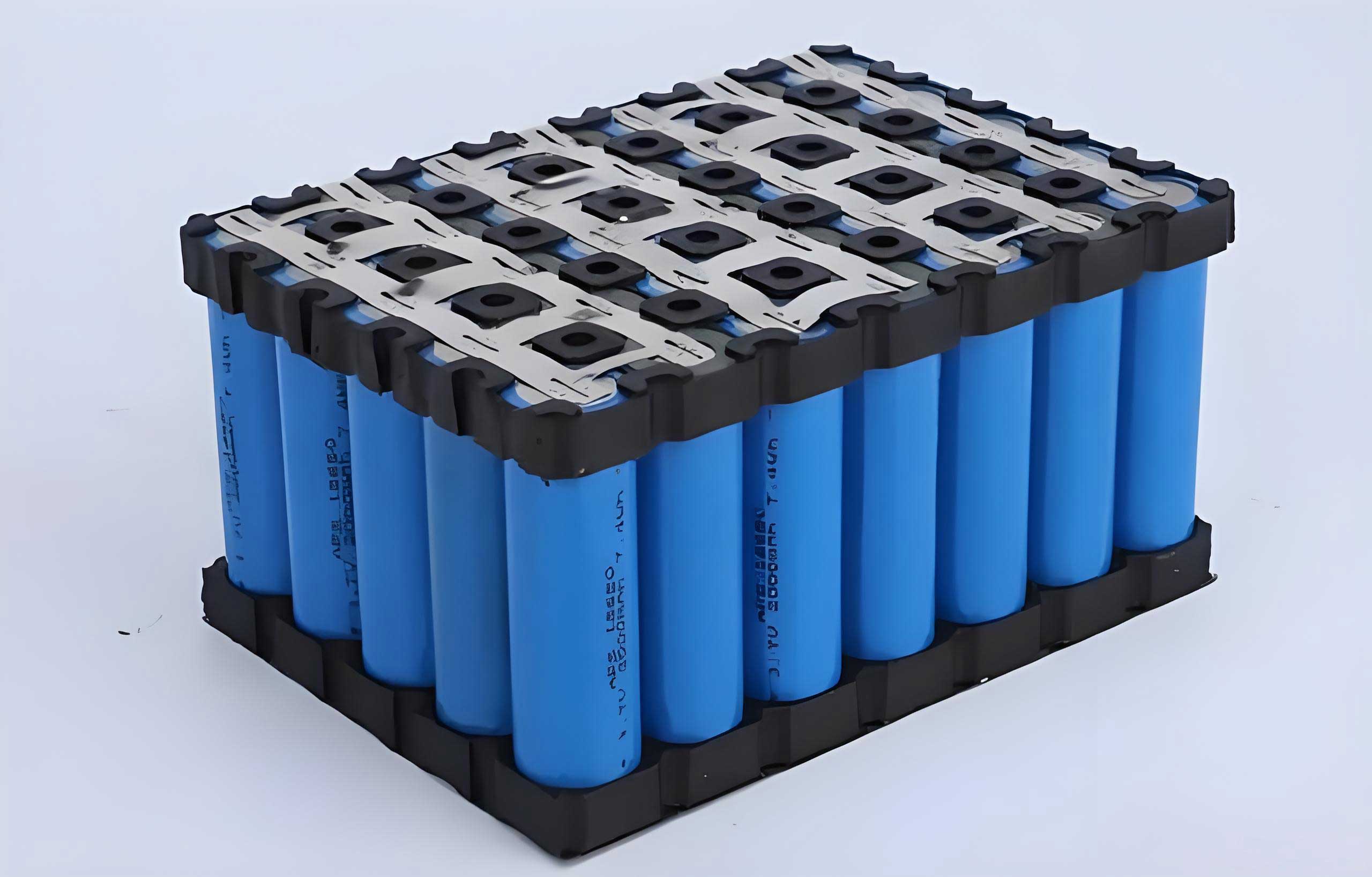
Existing methods for assessing LiFePO4 battery consistency often face limitations in balancing accuracy, computational complexity, and suitability for online, engineering-grade implementation. Some approaches rely heavily on empirically set thresholds, making them sensitive to specific operating conditions. Others, developed for electric vehicles, may not scale efficiently to handle the GB-level data streams from massive ESS. Techniques based on full voltage curve analysis or electrochemical impedance can be computationally intensive or require specialized testing protocols unsuitable for continuous online monitoring. This work proposes a pragmatic, integrated methodology designed for online deployment. It leverages the intrinsic charge/discharge characteristics of LiFePO4 battery clusters, employs a combination of robust statistical outlier detection algorithms for cross-validated problem identification, classifies the detected issues, and finally prioritizes them using an “optimization coefficient” derived from estimated capacity deviation, offering clear guidance for maintenance actions.
Operational Characteristics of LiFePO4 Battery Clusters in ESS and Foundational Principles
Modern utility-scale ESS are typically architected in a hierarchical manner: cells are integrated into modules, which are then connected to form battery clusters (strings), and clusters are combined into cabinets and systems. The battery cluster, as defined in standards like GB/T 36276, serves as a fundamental operational unit. This work focuses on the cluster level for analysis. The operational profile of a LiFePO4 battery cluster varies with its application. In “peak-shaving” mode, the charge and discharge cycles are typically diurnal, with low to moderate C-rates, emphasizing depth of discharge and capacity utilization. In “frequency regulation” mode, the cluster undergoes frequent but shallow charge-discharge cycles, with rapid power reversals.
A critical observation is that regardless of the application mode, the usable capacity of a cluster, \( Capacity_{used} \), is not merely the sum of individual cell capacities but is modulated by a consistency factor \( \alpha \) (where \( \alpha \leq 1 \)):
$$
Capacity_{used} = \alpha \cdot \sum Capacity_{single-battery}
$$
Directly measuring individual cell capacity online is impractical. However, inconsistency inevitably reveals itself through cell voltage divergence, especially during the charge and discharge endpoints. The flat voltage plateau characteristic of LiFePO4 chemistry during mid-SOC ranges makes voltage-based consistency assessment challenging in that region. Conversely, at the extremes of charge and discharge (i.e., at high and low SOC), the voltage exhibits a steeper slope. Here, even minor differences in cell state translate into measurable voltage differences, making these regions ideal for inconsistency detection.
Analysis of voltage data from clusters in both peak-shaving and frequency regulation applications confirms that the voltage deviation of each cell from the cluster’s average voltage (the “voltage delta”) at these global voltage extremes (maximum voltage during charge, minimum voltage during discharge) follows a statistical distribution. This distribution can be effectively modeled as a mixture of \( k \) Gaussian distributions:
$$
p(x_j) = \sum_{i=1}^{k} w_{i,j} \cdot \eta(x_j, \mu_{i,j}, \tau_{i,j})
$$
where \( \eta(x_j, \mu_{i,j}, \tau_{i,j}) \) is the probability density function of a Gaussian distribution:
$$
\eta(x_j, \mu_{i,j}, \tau_{i,j}) = \frac{1}{\sqrt{| \tau_{i,j} |}} e^{ -\frac{1}{2} (x_j – \mu_{i,j})^T \tau_{i,j}^{-1} (x_j – \mu_{i,j}) }
$$
and \( \tau_{i,j} = \delta_{i,j}^2 I \). Here, \( k \) represents the number of primary influencing factors (e.g., temperature gradients, inherent batch variance), \( w_{i,j} \) are the mixture weights, \( j \) denotes the condition type (charge-end or discharge-end), and \( I \) is the identity matrix. In an ideal, perfectly consistent pack with negligible influencing factors, the voltage deltas would cluster around zero, resembling a single Gaussian distribution \( N(0, \sigma^2) \). The presence of outlier cells or module-level imbalances manifests as additional, smaller peaks in this distribution.
Integrated Detection Model and Problem Classification Methodology
The proposed method is engineered for accuracy, simplicity, and low computational overhead. Its core is a hybrid outlier detection strategy applied to the voltage delta data at charge and discharge endpoints.
Hybrid Outlier Detection
1. Adjustable Gaussian Model (3σ Rule Adaptation): The standard Pauta (3σ) criterion for a normal distribution \( N(\mu, \sigma^2) \) states that approximately 99.73% of data lies within \( [\mu – 3\sigma, \mu + 3\sigma] \). Values outside this interval are considered rare outliers. For the mixture model describing our voltage deltas, the effective standard deviation is a composite measure. We adopt an adaptable threshold \( n \cdot \sigma_{eff} \), where \( \sigma_{eff} \) is the standard deviation of the empirical voltage delta dataset and \( n \) is a tunable parameter (typically starting near 3). A cell with a voltage delta satisfying \( |x – \mu| > n \cdot \sigma_{eff} \) is flagged as a preliminary outlier. The threshold \( n \) can be adjusted based on historical data and desired sensitivity, making the method less reliant on fixed empirical bounds.
2. Grubbs’ Test for Cross-Validation: To mitigate potential false positives from the Gaussian model and add statistical rigor, Grubbs’ test is employed concurrently. Grubbs’ test is designed to detect a single outlier in a dataset assumed to be normally distributed. For each potential outlier value \( x_{out} \), the test statistic \( G \) is calculated:
$$
G = \frac{|x_{out} – \bar{x}|}{s}
$$
where \( \bar{x} \) is the sample mean and \( s \) is the sample standard deviation. This \( G \) value is compared against a critical value \( G_{critical} \):
$$
G_{critical} = \frac{N-1}{\sqrt{N}} \sqrt{ \frac{ t_{\alpha/(2N), N-2}^2 }{ N-2 + t_{\alpha/(2N), N-2}^2 } }
$$
Here, \( N \) is the number of cells in the cluster, and \( t_{\alpha/(2N), N-2} \) is the critical value from the t-distribution with \( N-2 \) degrees of freedom and a significance level of \( \alpha/(2N) \) (for two-sided test). A cell is confirmed as an outlier if \( G > G_{critical} \). We apply two significance levels: a strict level (\( \alpha_1=0.005 \)) to identify “severe” outliers and a more relaxed level (\( \alpha_2=0.05 \)) to identify “moderate” outliers or potential precursors.
Problem Classification Logic
Cells flagged by the hybrid detection process are further classified based on their behavior at both charge and discharge endpoints. The classification logic is as follows:
Let \( U_p \) be the set of cells identified with abnormally high voltage deltas at the charge endpoint.
Let \( D_{own} \) be the set of cells identified with abnormally low voltage deltas at the discharge endpoint.
Let \( S_1 \) be the set of cells confirmed as “severe” outliers by Grubbs’ test (using \( \alpha_1 \)).
Let \( S_2 \) be the set of cells confirmed as “moderate” outliers by Grubbs’ test (using \( \alpha_2 \)).
The classification rules are algorithmically defined:
1. Potential Short-Board Set: \( DB = \{ j \, | \, j \in U_p \text{ and } j \in D_{own} \} \). A cell that is both high at charge-end and low at discharge-end exhibits the classic signature of a weak cell.
2. Confirmed Short-Board Cells: \( \text{ShortBoard} = (DB \cap S_2) \cup S_1 \). A cell in \( DB \) that is at least a moderate outlier, or any cell that is a severe outlier, is classified as a critical short-board cell requiring replacement.
3. Short-Board Trend Cells: Define intermediate sets \( A = D_{own} \cap S_2 \setminus \text{ShortBoard} \) and \( B = U_p \cap S_2 \setminus \text{ShortBoard} \). Then, \( \text{Trend} = A \cap B \). These cells show the signature but with weaker statistical strength, indicating early-stage degradation.
4. SOC Imbalance Cells: Cells showing inconsistency only at one endpoint: \( \text{HighImbalance} = A \setminus \text{Trend} \) (high at charge-end only), \( \text{LowImbalance} = B \setminus \text{Trend} \) (low at discharge-end only). These typically indicate cells that are out of sync with the cluster’s average SOC and might be correctable via balancing.
5. Module-Level Imbalance: If a majority of cells within a single physical module are classified as either \( \text{HighImbalance} \) or \( \text{LowImbalance} \), it is flagged as a module-level imbalance, potentially pointing to a faulty module sensor or connection.
Prioritization via Optimization Coefficient
Merely classifying problems is insufficient for efficient maintenance. A prioritization mechanism is essential. While ranking by voltage delta magnitude is simple, it is not comparable across different clusters with different average SOCs. A more informative metric is the estimated deviation capacity, which quantifies how much cluster capacity is currently being limited by the problematic cell.
The concept is illustrated using a charging curve. Assume cell \( X_1 \) is a short-board cell, reaching the charge cut-off voltage prematurely. Let \( X_2 \) be the cell with the highest voltage in the cluster at the charge endpoint, excluding \( X_1 \). We approximate that the voltage curve of \( X_1 \) is a shifted version of \( X_2 \)’s curve. The time shift \( \Delta t \) is the difference between the moment \( X_1 \) reaches the voltage level that \( X_2 \) has at the charge endpoint (\( t_1 \)) and the actual charge endpoint time (\( t_2 \)): \( \Delta t = t_2 – t_1 \).
The optimization coefficient \( \kappa \) (in Ah) is then the charge transferred during this period:
$$
\kappa = \int_{t_1}^{t_2} I_{cluster}(t) \, dt
$$
where \( I_{cluster}(t) \) is the cluster current. A larger positive \( \kappa \) for a short-board cell indicates a greater potential capacity recovery if that cell is replaced. For imbalance cells, \( |\kappa| \) represents the amount of charge misalignment. This coefficient provides a direct, actionable metric for maintenance crews to schedule interventions, focusing on cells with the highest \( \kappa \) values first.
Engineering Application and Validation
The proposed methodology was implemented and tested using operational data from a grid-scale LiFePO4 battery energy storage system performing peak-shaving duties. The system architecture consisted of battery clusters, each comprising multiple cells in series. The online monitoring system recorded cell voltages, cluster voltage and current, and temperatures at regular intervals.
The algorithm was configured with the following tunable parameters for the Gaussian filter and pre-filters:
| Parameter | Symbol | Value |
|---|---|---|
| Gaussian Sigma Multiplier | \( n \) | 2.800 |
| Charge-End High Voltage Filter | \( V_{s1} \) | 3.500 V |
| Discharge-End Low Voltage Filter | \( V_{s2} \) | 3.099 V |
| Minimum Delta for High Outlier | \( V_{s3} \) | 0.075 V |
| Minimum Delta for Low Outlier | \( V_{s4} \) | 0.075 V |
Applying the integrated detection and classification model to a representative 24-hour dataset from a specific cluster yielded the results summarized below. The analysis focused on the global voltage extremes during one complete charge-discharge cycle.
| Cluster Identifier | Cell ID | Problem Type | Max. High Delta (mV) | Max. Low Delta (mV) | Optimization Coef. \( \kappa \) (Ah) | Maintenance Suggestion |
|---|---|---|---|---|---|---|
| Cluster 3-1-1 | 5 | Short-Board | 176.1 | 305.9 | 2.64 | Priority Replacement |
| Cluster 3-1-1 | 48 | Low SOC Imbalance | -8.7 | 259.3 | -1* | Balancing Recommended |
| Cluster 3-2-3 | 211 | Short-Board | 152.1 | 279.9 | 2.22 | Replacement |
| Cluster 3-3-4 | 98 | Short-Board | 74.4 | 214.5 | 2.27 | Replacement |
* A coefficient of -1 indicates the presence of a more severe problem (Cell 5) in the same cluster; its calculation was superseded.
The results clearly identify specific problematic cells. For instance, in Cluster 3-1-1, Cell #5 was conclusively diagnosed as a short-board LiFePO4 battery cell, showing significant deviation at both endpoints and a high optimization coefficient, warranting immediate replacement. Cell #48 in the same cluster was identified as having a low SOC imbalance, a condition potentially correctable through the system’s balancing circuitry. The algorithm successfully distinguished between these fundamentally different issues. Validation through subsequent manual testing and maintenance logs confirmed the diagnoses, demonstrating a high identification accuracy rate (\( \mu \geq 99\% \)) and a high classification accuracy for short-board versus imbalance conditions (\( \alpha \geq 85\% \)). The computational load was minimal, suitable for real-time processing on edge devices within the ESS.
Conclusion
This work presents a practical, engineered solution for the online detection and diagnosis of inconsistencies in lithium iron phosphate battery energy storage systems. By leveraging the natural voltage characteristics of LiFePO4 batteries at charge/discharge endpoints and employing a hybrid statistical detection model combining an adaptable Gaussian filter with Grubbs’ test, the method achieves robust and accurate identification of outlier cells. Its novel classification logic effectively distinguishes between critical short-board LiFePO4 battery cells, incipient short-board trends, SOC imbalances, and module-level issues. The introduction of the optimization coefficient, derived from estimated capacity deviation, transforms qualitative alerts into a quantitative prioritization metric, directly guiding maintenance efficiency and maximizing return on intervention.
The methodology is characterized by its high accuracy, low computational complexity, and minimal dependence on hard-coded empirical thresholds due to its tunable parameters. These attributes make it exceptionally suitable for deployment in online monitoring systems of large-scale LiFePO4 battery ESS. It empowers operators to move from reactive to proactive maintenance, enhancing system safety, optimizing available capacity, and extending the overall service life of the energy storage asset. Future work will focus on enhancing the method’s predictive capabilities, using time-series analysis of the optimization coefficient and other features to forecast cell failures before they become critical, further solidifying the role of intelligent monitoring in the reliable operation of lithium iron phosphate battery fleets.