
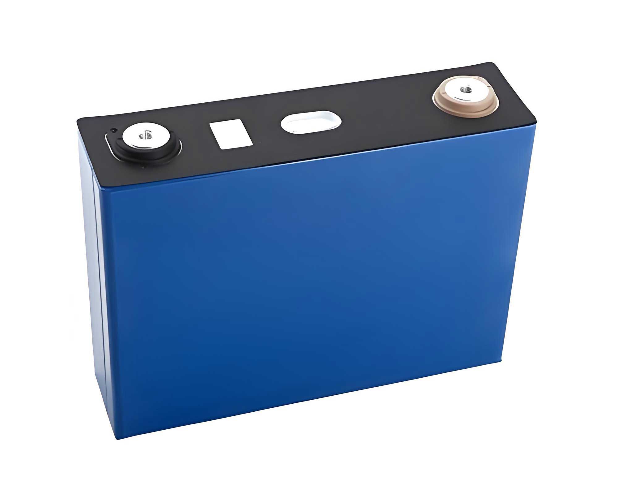
In the realm of electric vehicles, accurate estimation of the State of Charge (SOC) for power batteries is paramount for optimizing energy management, ensuring safety, and extending battery life. Among various battery types, the LiFePO4 battery stands out due to its high thermal stability, long cycle life, and enhanced safety profile. However, estimating SOC for LiFePO4 batteries poses challenges, particularly because of their flat voltage plateau in the mid-SOC range, which complicates model-based approaches. As an engineer focused on advancing battery management systems, I have explored methods to improve SOC estimation accuracy under dynamic driving conditions. This article presents a comprehensive approach that integrates online parameter identification with state estimation, specifically tailored for LiFePO4 batteries. The core innovation lies in dynamically optimizing the forgetting factor in recursive least squares algorithms using particle swarm optimization, thereby enhancing model fidelity and SOC estimation precision. Throughout this discussion, I will delve into the technical details, supported by mathematical formulations, tables, and simulation results, to underscore the efficacy of this method for LiFePO4 battery applications.
The foundation of any model-based SOC estimation strategy is an accurate equivalent circuit model that captures the battery’s electrochemical behavior. For LiFePO4 batteries, I adopt a second-order RC equivalent circuit model, which effectively represents dynamic responses such as polarization and diffusion effects. This model comprises an open-circuit voltage source, an ohmic resistor, and two RC parallel networks that account for electrochemical and concentration polarizations. The electrical dynamics can be described by Kirchhoff’s laws, leading to differential equations that govern terminal voltage behavior. Let me express this mathematically: the state variables include the voltages across the RC networks, denoted as $U_1(t)$ and $U_2(t)$, and the SOC, represented as $Z(t)$. The system input is the current $I(t)$, with discharge current considered positive. The terminal voltage $U_t(t)$ is given by:
$$U_t(t) = U_{oc}(Z) – U_1(t) – U_2(t) – I(t) \cdot R_0(t)$$
where $U_{oc}(Z)$ is the open-circuit voltage as a function of SOC, and $R_0(t)$ is the ohmic resistance. The dynamics of the RC networks are:
$$\dot{U}_1(t) = -\frac{U_1(t)}{R_1(t) C_1(t)} + \frac{I(t)}{C_1(t)}$$
$$\dot{U}_2(t) = -\frac{U_2(t)}{R_2(t) C_2(t)} + \frac{I(t)}{C_2(t)}$$
Here, $R_1(t)$ and $C_1(t)$ represent the electrochemical polarization resistance and capacitance, while $R_2(t)$ and $C_2(t)$ correspond to concentration polarization parameters. These parameters are time-varying due to factors like aging, temperature, and SOC changes, necessitating online identification for accurate modeling. For LiFePO4 batteries, this model structure is particularly suitable as it balances complexity and precision, enabling real-time implementation in battery management systems.
To relate SOC to measurable quantities, a reliable SOC-OCV relationship is essential. For LiFePO4 batteries, the OCV curve exhibits a flat region in the mid-SOC range, making polynomial fitting challenging. I conducted experimental tests under controlled conditions at 25°C, using a standardized procedure to obtain OCV points at various SOC levels. The battery was charged and discharged at a C-rate of 1/3, with sufficient rest periods to ensure equilibrium. The collected data points were then fitted using a sixth-order polynomial to capture the nonlinearities at low and high SOC values while maintaining accuracy in the flat region. The SOC-OCV function is expressed as:
$$U_{oc}(Z) = a_1 Z^6 + a_2 Z^5 + a_3 Z^4 + a_4 Z^3 + a_5 Z^2 + a_6 Z + a_7$$
where $Z$ is the SOC normalized between 0 and 1, and coefficients $a_1$ to $a_7$ are derived from least squares fitting. The table below summarizes these coefficients based on my experimental data for a typical LiFePO4 battery with a rated capacity of 100 Ah.
| Coefficient | Value |
|---|---|
| $a_1$ | -23.7 |
| $a_2$ | 86.9 |
| $a_3$ | -122.9 |
| $a_4$ | 84.5 |
| $a_5$ | -29.2 |
| $a_6$ | 4.9 |
| $a_7$ | 2.9 |
This fitted curve allows for accurate OV estimation from SOC, which is crucial for the equivalent circuit model. The LiFePO4 battery’s unique voltage characteristics underscore the importance of precise OCV modeling; even small errors can lead to significant SOC deviations due to the flat plateau.
Online parameter identification is critical for adapting the model to changing battery conditions. Traditional recursive least squares (RLS) methods suffer from data saturation when dealing with slow time-varying systems like LiFePO4 battery parameters. To mitigate this, I incorporate a forgetting factor $\lambda$ into the RLS algorithm, forming the Forgetting Factor Recursive Least Squares (FFRLS) method. The forgetting factor discounts older data, giving more weight to recent observations. However, selecting an optimal $\lambda$ is non-trivial; a fixed value may not suit all operational scenarios. Hence, I propose using Particle Swarm Optimization (PSO) to dynamically optimize $\lambda$ in real-time, termed PSO-FFRLS. The PSO algorithm searches for $\lambda$ that minimizes the terminal voltage error between model output and measured data, ensuring adaptive performance.
The discrete-time representation of the equivalent circuit model is derived via bilinear transformation. Defining the parameter vector $\boldsymbol{\theta}(k) = [\theta_1, \theta_2, \theta_3, \theta_4, \theta_5]^T$ and data vector $\boldsymbol{\phi}(k) = [y(k-1), y(k-2), I(k), I(k-1), I(k-2)]^T$, where $y(k) = U_t(k) – U_{oc}(k)$, the system equation is:
$$y(k) = \boldsymbol{\theta}^T(k) \boldsymbol{\phi}(k)$$
The FFRLS update equations are:
$$\mathbf{K}(k) = \frac{\mathbf{P}(k-1) \boldsymbol{\phi}(k)}{\lambda + \boldsymbol{\phi}^T(k) \mathbf{P}(k-1) \boldsymbol{\phi}(k)}$$
$$\mathbf{P}(k) = \frac{1}{\lambda} \left[ \mathbf{I} – \mathbf{K}(k) \boldsymbol{\phi}^T(k) \right] \mathbf{P}(k-1)$$
$$\boldsymbol{\theta}(k) = \boldsymbol{\theta}(k-1) + \mathbf{K}(k) \left[ U_t(k) – U_{oc}(k) – \boldsymbol{\theta}^T(k-1) \boldsymbol{\phi}(k) \right]$$
where $\mathbf{K}(k)$ is the gain matrix, $\mathbf{P}(k)$ is the covariance matrix, and $\lambda$ is the forgetting factor. In PSO-FFRLS, a swarm of particles represents candidate $\lambda$ values, and the fitness function is the absolute terminal voltage error:
$$J = |U_t(k) – U(k)| = |U_t(k) – \boldsymbol{\theta}^T(k-1) \boldsymbol{\phi}(k) – U_{oc}(k-1)|$$
PSO iteratively updates particle positions and velocities to find $\lambda$ that minimizes $J$. This dynamic optimization allows the LiFePO4 battery model to adapt to varying conditions, such as load changes or temperature fluctuations, enhancing parameter identification accuracy.
For SOC estimation, I combine the online identified model with the Extended Kalman Filter (EKF), a powerful tool for nonlinear state estimation. The EKF linearizes the system around the current state estimate, enabling recursive updates. The state vector is $\mathbf{x}(k) = [U_1(k), U_2(k), Z(k)]^T$, with input $u(k) = I(k)$ and output $h(k) = U_t(k)$. The discrete state-space model is:
$$\mathbf{x}(k+1) = \mathbf{A}(k) \mathbf{x}(k) + \mathbf{B}(k) u(k) + \boldsymbol{\omega}(k)$$
$$U_t(k) = \mathbf{C}(k) \mathbf{x}(k) + \mathbf{D}(k) u(k) + \nu(k)$$
where $\boldsymbol{\omega}(k)$ and $\nu(k)$ are process and measurement noises, assumed Gaussian with zero mean. The matrices $\mathbf{A}(k)$, $\mathbf{B}(k)$, $\mathbf{C}(k)$, and $\mathbf{D}(k)$ are derived from linearizing the continuous-time dynamics, incorporating the identified parameters $R_0$, $R_1$, $R_2$, $C_1$, and $C_2$ from PSO-FFRLS. Specifically:
$$\mathbf{A}(k) = \begin{bmatrix} e^{-\frac{T}{R_1 C_1}} & 0 & 0 \\ 0 & e^{-\frac{T}{R_2 C_2}} & 0 \\ 0 & 0 & 1 \end{bmatrix}$$
$$\mathbf{B}(k) = \begin{bmatrix} R_1 \left(1 – e^{-\frac{T}{R_1 C_1}}\right) \\ R_2 \left(1 – e^{-\frac{T}{R_2 C_2}}\right) \\ -\frac{\eta T}{C_N} \end{bmatrix}$$
$$\mathbf{C}(k) = \begin{bmatrix} -1 & -1 & \frac{\partial U_{oc}(Z)}{\partial Z} \bigg|_{Z=Z(k)} \end{bmatrix}$$
$$\mathbf{D}(k) = -R_0$$
Here, $T$ is the sampling period, $\eta$ is the coulombic efficiency, and $C_N$ is the battery capacity. The EKF algorithm involves prediction and correction steps. The prediction step computes the a priori state estimate and error covariance:
$$\hat{\mathbf{x}}(k|k-1) = \mathbf{A}(k) \hat{\mathbf{x}}(k-1|k-1) + \mathbf{B}(k) u(k-1)$$
$$\mathbf{P}_e(k|k-1) = \mathbf{Q}(k-1) + \mathbf{A}(k-1) \mathbf{P}_e(k-1|k-1) \mathbf{A}^T(k-1)$$
where $\mathbf{Q}$ is the process noise covariance matrix. The correction step updates the estimate based on the measurement:
$$\mathbf{K}_e(k) = \mathbf{P}_e(k|k-1) \mathbf{C}^T(k) \left[ \mathbf{C}(k) \mathbf{P}_e(k|k-1) \mathbf{C}^T(k) + \mathbf{R}(k) \right]^{-1}$$
$$\hat{\mathbf{x}}(k|k) = \hat{\mathbf{x}}(k|k-1) + \mathbf{K}_e(k) \left[ U_t(k) – \mathbf{C}(k) \hat{\mathbf{x}}(k|k-1) \right]$$
$$\mathbf{P}_e(k|k) = \left[ \mathbf{I} – \mathbf{K}_e(k) \mathbf{C}(k) \right] \mathbf{P}_e(k|k-1)$$
with $\mathbf{R}$ as the measurement noise covariance matrix. By integrating PSO-FFRLS for parameter identification and EKF for state estimation, the SOC of LiFePO4 batteries can be estimated with high accuracy even under dynamic operating conditions.
To validate the proposed method, I conducted experiments using a commercial LiFePO4 battery cell with a nominal capacity of 100 Ah and voltage of 3.2 V. The test setup included a battery cycler, temperature chamber, and data acquisition system. Dynamic Stress Test (DST) profiles were applied to emulate real driving cycles, with current and voltage recorded at 1-second intervals. The DST cycle lasts 360 seconds, and multiple cycles were run to discharge the battery from 100% to 10% SOC. This data serves as the basis for simulation and analysis. In simulations, I implemented the PSO-FFRLS-EKF algorithm in MATLAB, comparing it against fixed-forgetting-factor FFRLS-EKF approaches with $\lambda = 0.95$ and $\lambda = 0.99$. The PSO parameters were set with a swarm size of 20, and $\lambda$ was constrained between 0.98 and 1.00 based on preliminary trials for LiFePO4 batteries.
The online identification performance was evaluated by terminal voltage error. The table below summarizes the error statistics for different methods over the entire DST test.
| Method | Maximum Voltage Error (mV) | Average Voltage Error (mV) |
|---|---|---|
| Fixed $\lambda = 0.95$ | 23.0 | 7.14 |
| Fixed $\lambda = 0.99$ | 13.1 | 2.78 |
| Dynamic $\lambda$ (PSO-FFRLS) | 12.3 | 2.18 |
Clearly, the dynamic forgetting factor approach yields the lowest errors, demonstrating its superiority in adapting to the LiFePO4 battery’s behavior. The voltage estimation closely tracks the measured data, ensuring a reliable model for SOC estimation.
For SOC estimation, the results are equally compelling. The reference SOC was calculated using coulomb counting with high-precision current integration. The estimation errors for each method are tabulated below.
| Method | Maximum SOC Error (%) | Average SOC Error (%) |
|---|---|---|
| Fixed $\lambda = 0.95$ with EKF | 4.05 | 1.59 |
| Fixed $\lambda = 0.99$ with EKF | 1.97 | 1.18 |
| PSO-FFRLS with EKF | 1.48 | 0.92 |
The PSO-FFRLS-EKF method achieves the highest accuracy, with an average SOC error below 1%. This is significant for LiFePO4 battery management, as even small errors can impact vehicle range and battery health. The dynamic optimization of $\lambda$ allows the algorithm to handle the flat voltage plateau effectively, reducing drift and improving convergence. Moreover, the computational load of PSO is manageable for real-time implementation, given the slow parameter variations in LiFePO4 batteries.
In conclusion, the integration of particle swarm optimization with forgetting factor recursive least squares and extended Kalman filtering presents a robust solution for SOC estimation in LiFePO4 batteries. The key innovation—dynamic optimization of the forgetting factor—ensures that the model parameters are accurately identified online, adapting to changes in battery dynamics. This method addresses the limitations of fixed forgetting factors, which may not suit all operating conditions, especially for LiFePO4 batteries with their unique voltage characteristics. Experimental results under dynamic stress tests confirm that the proposed approach reduces terminal voltage errors and enhances SOC estimation accuracy compared to conventional methods. For practical applications in electric vehicles, this algorithm can be embedded in battery management systems to improve reliability and performance. Future work may explore hybridization with other metaheuristic algorithms or extension to battery state-of-health estimation. Ultimately, advancing SOC estimation techniques for LiFePO4 batteries contributes to the broader adoption of electric vehicles by ensuring efficient and safe battery operation.