
In my extensive research and development work on renewable energy systems, I have focused on the critical technologies required for high-power solar inverters. These inverters are essential for converting the direct current generated by photovoltaic panels into alternating current suitable for grid integration. Over the years, I have tackled numerous challenges related to efficiency, stability, and grid compliance, leading to the implementation of robust control strategies. In this article, I will share my insights and experiences on key aspects such as maximum power point tracking (MPPT), low-voltage ride-through (LVRT), and anti-islanding detection, all crucial for the reliable operation of solar inverters in large-scale photovoltaic plants.
The proliferation of solar energy has necessitated the development of advanced solar inverters capable of handling high power levels while maintaining grid standards. My work primarily involves non-isolated single-stage three-phase grid-connected solar inverters, which offer high efficiency and compact design. The topology typically includes solar panels, DC-link capacitors, a three-phase full-bridge inverter, and an LCL filter. The control system must address functional requirements like MPPT and LVRT, as well as performance metrics such as power factor and harmonic distortion. Throughout my research, I have developed a comprehensive control framework based on positive and negative sequence decomposition to enhance the robustness of solar inverters under various grid conditions.
One of the core challenges in solar inverters is maximizing energy harvest from photovoltaic arrays under varying environmental conditions. I have implemented a fast variable-step perturbation and observation (P&O) MPPT algorithm combined with power prediction to address misjudgment issues during optimization. Traditional MPPT methods often struggle with rapid changes in irradiation or partial shading, leading to power losses. My approach adjusts the perturbation step size dynamically based on power variations, improving tracking speed and accuracy. The algorithm can be summarized with the following formulas and a comparison table of MPPT techniques.
The power output of a solar panel can be modeled using the characteristic equation:
$$P = V \times I$$
where \(P\) is power, \(V\) is voltage, and \(I\) is current. The MPPT algorithm aims to find the voltage \(V_{mp}\) that maximizes \(P\). In my variable-step P&O method, the perturbation step size \(\Delta V\) is adjusted according to:
$$\Delta V = k \times \left| \frac{P_k – P_{k-1}}{V_k – V_{k-1}} \right|$$
where \(k\) is a scaling factor, and \(P_k\) and \(V_k\) are the power and voltage at the current sampling instant. To prevent misjudgment due to noise or fluctuations, I incorporate power prediction by estimating the next power value \(P’_{k+1}\) as:
$$P’_{k+1} = 2P_{k+1/2} – P_k$$
where \(P_{k+1/2}\) is an intermediate power measurement. This allows the solar inverter to quickly adapt to changing conditions while maintaining stability.
| MPPT Method | Advantages | Disadvantages | Suitability for Solar Inverters |
|---|---|---|---|
| Perturb and Observe | Simple implementation | Oscillations around MPP | Moderate |
| Incremental Conductance | High accuracy | Computationally intensive | High |
| Variable-Step P&O with Prediction | Fast response, reduced misjudgment | Requires additional sensing | Very High |
In my experiments with a 500 kW solar inverter platform, this MPPT strategy demonstrated excellent performance under partial shading conditions. The solar inverter swiftly adjusted the operating point to track the global maximum power, ensuring minimal energy loss. The dynamic response was validated through waveforms showing voltage and current transitions during shading events, confirming the effectiveness of the algorithm for high-power solar inverters.
Another critical aspect for grid-connected solar inverters is low-voltage ride-through (LVRT), which requires the inverter to remain connected during grid voltage sags. I have developed an LVRT control strategy based on positive and negative sequence current decomposition to suppress negative sequence currents and maintain power quality. During voltage dips, the solar inverter must provide reactive power support while limiting overcurrents. My approach involves dual-loop control with an outer voltage loop for power regulation and an inner current loop for grid current tracking.
When the grid voltage becomes unbalanced due to faults, the three-phase quantities can be decomposed into symmetric components. The active and reactive power outputs can be expressed as:
$$\begin{bmatrix} P_0 \\ Q_0 \\ P_a \\ P_b \end{bmatrix} = \frac{3}{2} \begin{bmatrix} e_d^+ & e_q^+ & e_d^- & e_q^- \\ e_q^+ & -e_d^+ & e_q^- & -e_d^- \\ e_d^- & e_q^- & e_d^+ & e_q^+ \\ e_q^- & -e_d^- & e_q^+ & -e_d^+ \end{bmatrix} \begin{bmatrix} i_d^+ \\ i_q^+ \\ i_d^- \\ i_q^- \end{bmatrix}$$
where \(e\) and \(i\) represent voltage and current components in the dq-frame, with superscripts \(+\) and \(-\) denoting positive and negative sequences. To achieve LVRT compliance, I set the negative sequence current reference to zero to minimize unbalance, while the positive sequence current references are constrained by:
$$\sqrt{(i_d^+)^2 + (i_q^+)^2} \leq I_{\text{max}}$$
where \(I_{\text{max}}\) is the inverter’s current limit. The reactive power reference \(Q_{\text{ref}}\) is adjusted based on the voltage dip depth to provide grid support, following grid code requirements.
I implemented this strategy in a 500 kW solar inverter, testing it under balanced and unbalanced voltage sags down to 20% of nominal voltage. The solar inverter successfully maintained connection without overcurrent, and the current waveforms remained sinusoidal with low distortion. The transition times and power recovery met the standards, showcasing the robustness of the LVRT control for solar inverters in fault conditions.
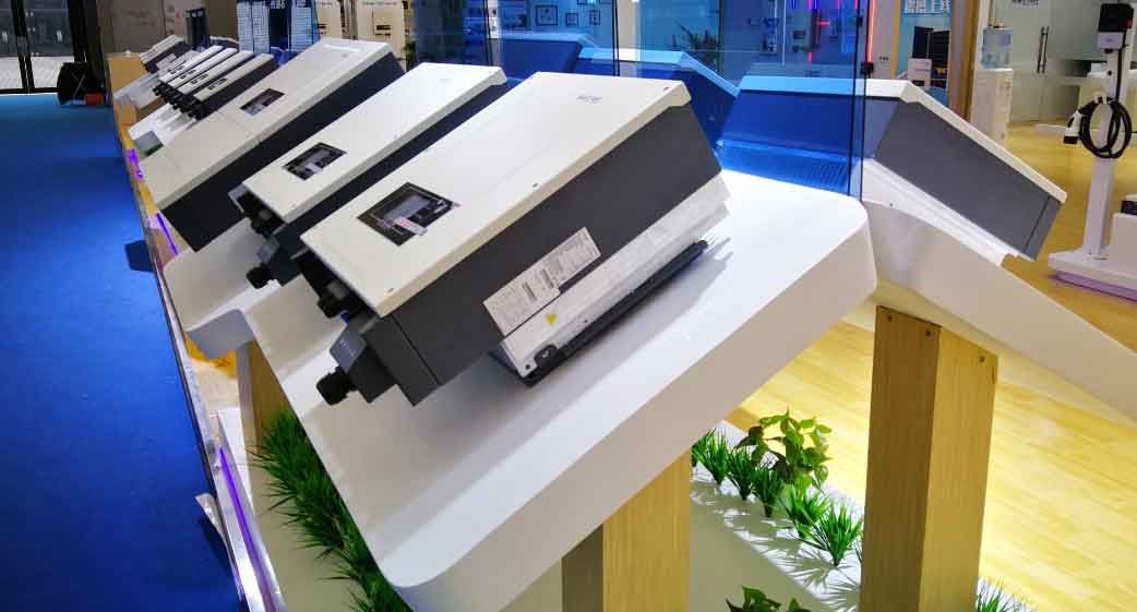
Integration of energy storage systems with solar inverters is becoming increasingly important for grid stability, as shown in the image above. This complements the LVRT capabilities by providing additional power buffer during faults, enhancing the reliability of solar inverters in modern power networks.
Anti-islanding detection is a safety requirement for solar inverters to prevent unintended operation when the grid is disconnected. I have adopted an active detection method based on reactive power disturbance, which minimally impacts power quality while ensuring fast detection. In islanding conditions, the voltage and frequency at the point of common coupling (PCC) can deviate, posing risks to maintenance personnel and equipment. My method injects a small reactive current perturbation at regular intervals to destabilize the islanded system.
The relationship between PCC frequency \(f\) and reactive current \(i_q\) can be derived from the load dynamics. For a parallel RLC load, the frequency deviation \(\Delta f\) is given by:
$$\Delta f = \frac{1}{2\pi} \cdot \frac{i_q \cdot V_{\text{pcc}}}{P_{\text{load}}} \cdot Q_f$$
where \(V_{\text{pcc}}\) is the PCC voltage, \(P_{\text{load}}\) is the load power, and \(Q_f\) is the quality factor. By injecting a reactive current disturbance of \(\Delta i_q = 0.05\) per unit, the frequency can be driven outside the normal range (e.g., 49.5 Hz to 50.3 Hz), triggering islanding detection. I implement this by modulating the q-axis current reference in the control loop every 20 grid cycles, with each disturbance lasting two cycles. This approach balances detection speed and grid current quality for solar inverters.
In my tests, the solar inverter detected islanding within 41.2 ms for a load with a quality factor of 0.989, well under the 2-second requirement. The grid current distortion during normal operation was negligible, demonstrating the practicality of this method for high-power solar inverters. The following table summarizes key parameters for anti-islanding detection in solar inverters.
| Parameter | Value | Description |
|---|---|---|
| Detection Time | < 2 s | Grid code requirement |
| Reactive Current Disturbance | 5% of rated | Minimizes power quality impact |
| Disturbance Interval | Every 20 cycles | Balances sensitivity and stability |
| Load Quality Factor Range | Up to 2.5 | Covers typical scenarios |
The overall control strategy for solar inverters integrates these technologies into a unified system. I use a dual-loop structure with grid voltage feedforward and capacitor current feedback to enhance dynamic performance and damp LCL filter resonance. The current loop employs proportional-integral (PI) regulators in the dq-frame, with separate controllers for positive and negative sequences. The modulation signals are generated via space vector pulse-width modulation (SVPWM) to drive the inverter switches efficiently.
For a 500 kW solar inverter with parameters like DC-link voltage of 900 V and grid voltage of 270 V, I achieved a power factor exceeding 0.999 and total harmonic distortion (THD) below 1.67% at full power. The average efficiency was around 97%, meeting national standards. These results underscore the effectiveness of my control approaches for solar inverters in real-world applications.
To further elaborate on the system modeling, the dynamics of the solar inverter can be described using state-space equations. The LCL filter introduces resonance at frequency \(\omega_r\), given by:
$$\omega_r = \frac{1}{\sqrt{L_1 C_f}}$$
where \(L_1\) is the inverter-side inductance and \(C_f\) is the filter capacitance. To mitigate this, I implement active damping by feeding back the capacitor current \(i_c\) with a gain \(K_d\):
$$i_{\text{ref, damp}} = K_d \cdot i_c$$
This modifies the current reference to suppress oscillations, ensuring stability for solar inverters without sacrificing efficiency.
In terms of grid synchronization, I employ a phase-locked loop (PLL) based on positive sequence extraction to accurately track grid angle even under unbalanced conditions. The PLL dynamics can be modeled as:
$$\frac{d\theta}{dt} = \omega_{\text{grid}} + K_p \cdot e_{\theta} + K_i \cdot \int e_{\theta} dt$$
where \(\theta\) is the estimated phase angle, \(\omega_{\text{grid}}\) is the grid frequency, and \(e_{\theta}\) is the phase error. This ensures robust performance for solar inverters during grid disturbances.
Looking ahead, the evolution of solar inverters will involve greater integration with smart grid functionalities, such as virtual inertia and frequency regulation. My research continues to explore adaptive control algorithms that can optimize solar inverter performance in real-time based on grid conditions. For instance, machine learning techniques could be applied to predict solar irradiation patterns and pre-adjust MPPT parameters, further enhancing energy yield.
In conclusion, the development of high-power solar inverters requires a holistic approach to control design, addressing MPPT, LVRT, and anti-islanding simultaneously. My experiences demonstrate that through advanced sequencing and predictive strategies, solar inverters can achieve high efficiency, reliability, and grid compliance. The key is to balance dynamic response with stability, ensuring that solar inverters contribute positively to the renewable energy landscape. As solar penetration increases, these technologies will play a pivotal role in maintaining power system integrity and enabling a sustainable energy future.
To summarize the formulas and key points discussed, here is a comprehensive list of equations relevant to solar inverters:
1. MPPT power relation: $$P = V \times I$$
2. Variable-step perturbation: $$\Delta V = k \times \left| \frac{\Delta P}{\Delta V} \right|$$
3. Power prediction: $$P’_{k+1} = 2P_{k+1/2} – P_k$$
4. Positive-negative sequence power decomposition: $$\begin{bmatrix} P_0 \\ Q_0 \end{bmatrix} = \frac{3}{2} \begin{bmatrix} e_d^+ & e_q^+ \\ e_q^+ & -e_d^+ \end{bmatrix} \begin{bmatrix} i_d^+ \\ i_q^+ \end{bmatrix} + \frac{3}{2} \begin{bmatrix} e_d^- & e_q^- \\ e_q^- & -e_d^- \end{bmatrix} \begin{bmatrix} i_d^- \\ i_q^- \end{bmatrix}$$
5. Current limit constraint: $$\sqrt{(i_d^+)^2 + (i_q^+)^2} \leq I_{\text{max}}$$
6. Islanding frequency deviation: $$\Delta f = \frac{1}{2\pi} \cdot \frac{i_q \cdot V_{\text{pcc}}}{P_{\text{load}}} \cdot Q_f$$
7. LCL resonance frequency: $$\omega_r = \frac{1}{\sqrt{L_1 C_f}}$$
8. Active damping feedback: $$i_{\text{ref, damp}} = K_d \cdot i_c$$
9. PLL dynamics: $$\frac{d\theta}{dt} = \omega_{\text{grid}} + K_p \cdot e_{\theta} + K_i \cdot \int e_{\theta} dt$$
These equations form the mathematical foundation for the control strategies implemented in modern solar inverters. By continuously refining these models and algorithms, I aim to push the boundaries of what solar inverters can achieve, contributing to more efficient and resilient power systems globally.